Multiple CRS in one axis

This is an example of how you can use multiple CRS in one plot.

using CairoMakie, GeoMakie
using Rasters, RasterDataSources, ArchGDAL

ras = Raster(EarthEnv{HabitatHeterogeneity}, :homogeneity)

╭───────────────────────────────────────╮
│ 1728×696 Raster{UInt16,2} homogeneity │
├───────────────────────────────────────┴──────────────────────────────── dims ┐
  ↓ X Projected{Float64} LinRange{Float64}(-180.0, 179.79166666666669, 1728) ForwardOrdered Regular Intervals{Start},
  → Y Projected{Float64} LinRange{Float64}(84.79166666666667, -60.0, 696) ReverseOrdered Regular Intervals{Start}
├──────────────────────────────────────────────────────────────────── metadata ┤
  Metadata{Rasters.GDALsource} of Dict{String, Any} with 4 entries:
  "units"    => ""
  "offset"   => 0.0
  "filepath" => "/home/runner/.julia/artifacts/EarthEnv/HabitatHeterogeneity/25…
  "scale"    => 1.0
├────────────────────────────────────────────────────────────────────── raster ┤
  extent: Extent(X = (-180.0, 180.00000000000003), Y = (-60.0, 85.0))
  missingval: 0xffff
  crs: GEOGCS["WGS 84",DATUM["WGS_1984",SPHEROID["WGS 84",6378137,298.257223563,AUTHORITY["EPSG","7030"]],AUTHORITY["EPSG","6326"]],PRIMEM["Greenwich",0,AUTHORITY["EPSG","8901"]],UNIT["degree",0.0174532925199433,AUTHORITY["EPSG","9122"]],AXIS["Latitude",NORTH],AXIS["Longitude",EAST],AUTHORITY["EPSG","4326"]]
└──────────────────────────────────────────────────────────────────────────────┘
    ↓ →        84.7917      84.5833  …     -59.5833     -59.7917     -60.0
 -180.0    0xffff       0xffff          0xffff       0xffff       0xffff
    ⋮                                ⋱                    ⋮       
  179.792  0xffff       0xffff          0xffff       0xffff       0xffff

heatmap(ras; axis = (; aspect = DataAspect()))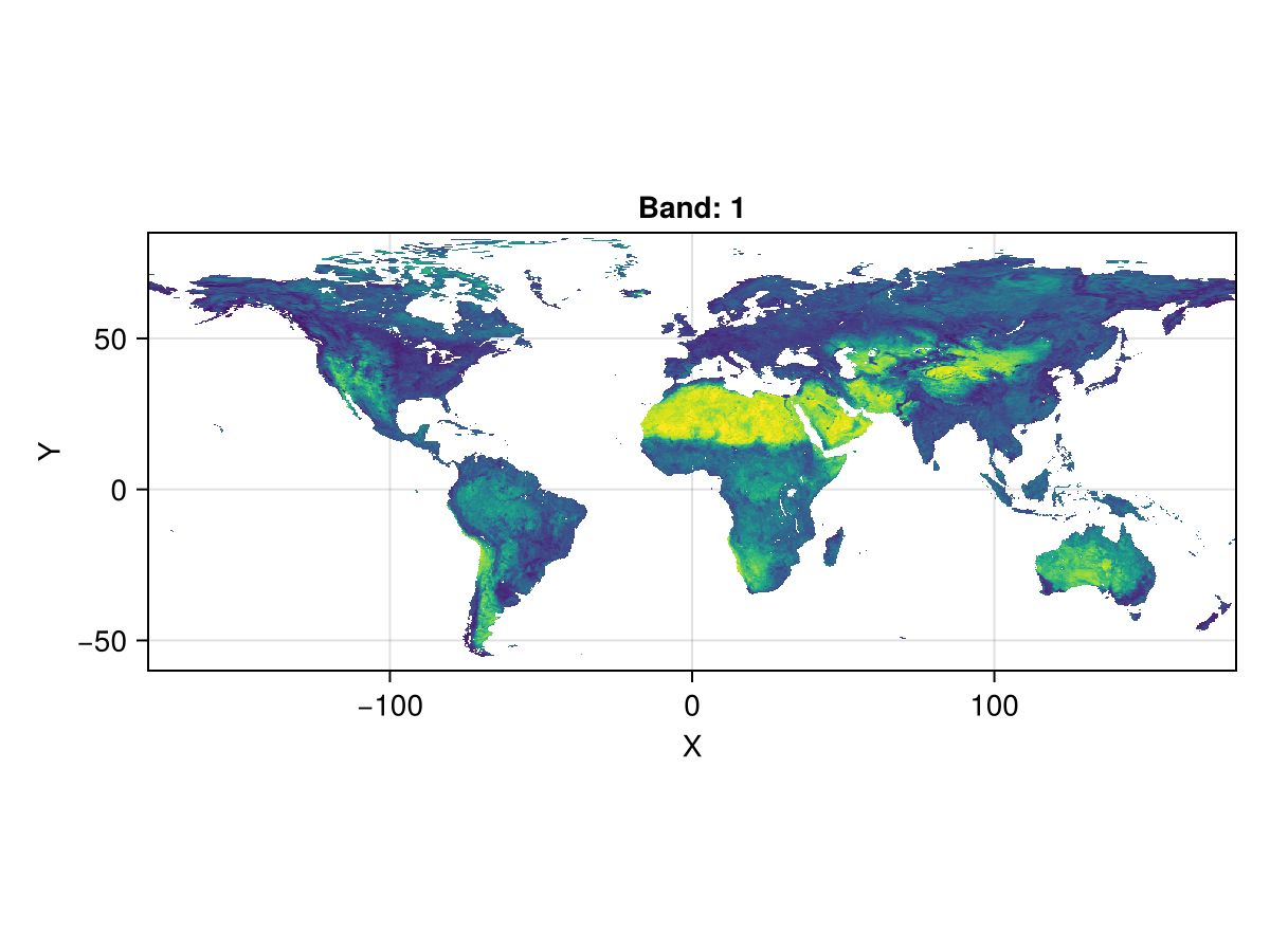

Let's simulate a new CRS, assuming this was an image taken from a geostationary satellite, hovering above 72° E:

projected_ras = Rasters.warp(
        ras,
        Dict(
            "s_srs" => convert(GeoFormatTypes.ProjString, Rasters.crs(ras)).val, # source CRS
            "t_srs" => "+proj=geos +h=3578600 +lon_0=72" # the CRS to which this should be transformed
        )
    )

╭────────────────────────────────────────╮
│ 1320×1315 Raster{UInt16,2} homogeneity │
├────────────────────────────────────────┴─────────────────────────────── dims ┐
  ↓ X Projected{Float64} LinRange{Float64}(-2.486249645439198e6, 2.482616027312147e6, 1320) ForwardOrdered Regular Intervals{Start},
  → Y Projected{Float64} LinRange{Float64}(2.4773207062691883e6, -2.472709236107815e6, 1315) ReverseOrdered Regular Intervals{Start}
├──────────────────────────────────────────────────────────────────── metadata ┤
  Metadata{Rasters.GDALsource} of Dict{String, Any} with 4 entries:
  "units"    => ""
  "offset"   => 0.0
  "filepath" => "/vsimem/tmp"
  "scale"    => 1.0
├────────────────────────────────────────────────────────────────────── raster ┤
  extent: Extent(X = (-2.486249645439198e6, 2.4863831733870152e6), Y = (-2.472709236107815e6, 2.4810878523440566e6))
  missingval: 0xffff
  crs: PROJCS["unknown",GEOGCS["unknown",DATUM["WGS_1984",SPHEROID["WGS 84",6378137,298.257223563,AUTHORITY["EPSG","7030"]],AUTHORITY["EPSG","6326"]],PRIMEM["Greenwich",0,AUTHORITY["EPSG","8901"]],UNIT["degree",0.0174532925199433,AUTHORITY["EPSG","9122"]]],PROJECTION["Geostationary_Satellite"],PARAMETER["central_meridian",72],PARAMETER["satellite_height",3578600],PARAMETER["false_easting",0],PARAMETER["false_northing",0],UNIT["metre",1,AUTHORITY["EPSG","9001"]],AXIS["Easting",EAST],AXIS["Northing",NORTH]]
└──────────────────────────────────────────────────────────────────────────────┘
  ↓ →             2.47732e6  …      -2.46894e6      -2.47271e6
 -2.48625e6  0xffff             0xffff          0xffff
  ⋮                          ⋱       ⋮          
  2.48262e6  0xffff             0xffff          0xffff

This is what the raster would look like, if it were taken directly from a satellite image:

heatmap(projected_ras; axis = (; aspect = DataAspect()))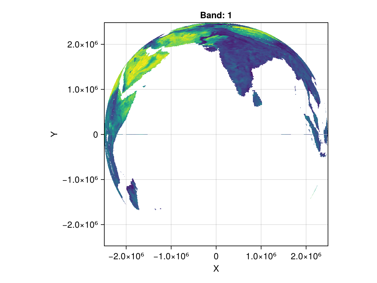

Now, we can create a GeoAxis with coastlines in the equal earth projection:

fig = Figure()
ga = GeoAxis(fig[1, 1])
lines!(ga, GeoMakie.coastlines())
fig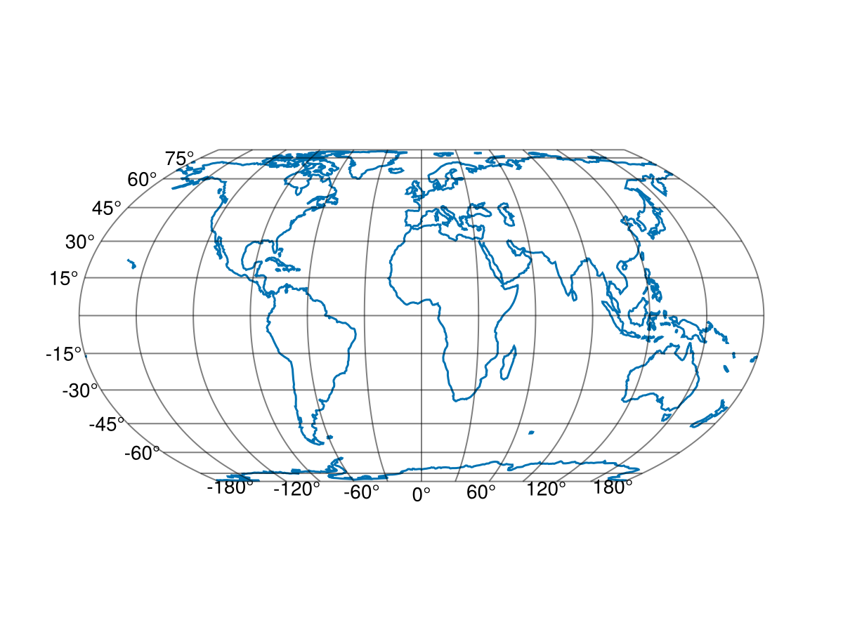

The coastlines function returns points in the (lon, lat) coordinate reference system.

We will now plot our image, from the geostationary coordinate system:

heatmap!(ga, projected_ras)
fig

Success! You can clearly see how the raster was adapted here.

---

This page was generated using Literate.jl.