Streamplot
This example was translated from the Cartopy streamplot example.
julia
using CairoMakie, GeoMakie
using Interpolations # for Streamplot on gridded data if necessary

f(x::Point2{T}) where T = Point2{T}(
    10 * (2 * cos(2 * deg2rad(x[1]) + 3 * deg2rad(x[2] + 30)) ^ 2),
    20 * cos(6 * deg2rad(x[1]))
)

pole_longitude=177.5
pole_latitude=37.5
fig, ax, plt = streamplot(
    f, 311.9..391.1, -23.6..24.8;
    arrow_size = 6,
    source = "+proj=ob_tran +o_proj=latlon +o_lon_p=0 +o_lat_p=$(pole_latitude) +lon_0=$(180+pole_longitude) +to_meter=$(deg2rad(1) * 6378137.0)",
    axis = (;
        type = GeoAxis,
        title = "Streamplot",
    )
)
lp = lines!(ax, GeoMakie.coastlines(); linewidth = 0.5, color = :black, xautolimits = false, yautolimits = false)
translate!(lp, 0, 0, -1)
fig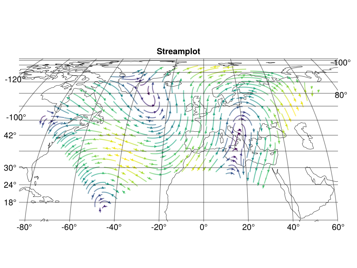
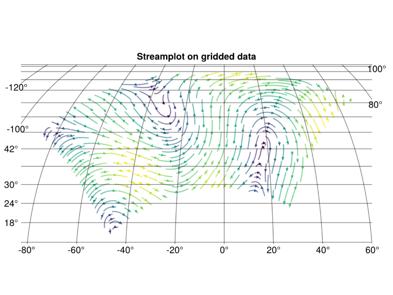
Gridded data
You can also do a streamplot on gridded data via Interpolations.jl:
julia
using Interpolations
xs = range(311.9, 391.1, 100)
ys = range(-23.6, 24.8, 100)
uvs = f.(Point2f.(xs, ys'))
100×100 Matrix{GeometryBasics.Point{2, Float32}}:
[1.01205, 6.37921] [1.24817, 6.37921] … [2.75829, 6.37921]
[1.27078, 4.77064] [1.53188, 4.77064] [2.38461, 4.77064]
[1.55672, 3.12869] [1.84199, 3.12869] [2.03471, 3.12869]
[1.86898, 1.46479] [2.17753, 1.46479] [1.70964, 1.46479]
[2.20662, -0.209463] [2.5375, -0.209463] [1.4104, -0.209463]
[2.56855, -1.88217] [2.92071, -1.88217] … [1.13797, -1.88217]
[2.95365, -3.54167] [3.32601, -3.54167] [0.893167, -3.54167]
[3.36074, -5.17641] [3.75212, -5.17641] [0.676764, -5.17641]
[3.78851, -6.77476] [4.1977, -6.77476] [0.489441, -6.77476]
[4.23567, -8.3256] [4.66139, -8.3256] [0.33177, -8.3256]
⋮ ⋱
[2.66271, -16.9979] [2.32462, -16.9979] [13.8107, -16.9979]
[2.29487, -17.8201] [1.97876, -17.8201] [13.2887, -17.8201]
[1.95107, -18.5174] [1.65794, -18.5174] [12.7564, -18.5174]
[1.63235, -19.0848] [1.3631, -19.0848] [12.2155, -19.0848]
[1.33975, -19.5183] [1.09522, -19.5183] … [11.6677, -19.5183]
[1.07414, -19.815] [0.855103, -19.815] [11.1147, -19.815]
[0.836372, -19.9726] [0.643502, -19.9726] [10.5582, -19.9726]
[0.627185, -19.9901] [0.461085, -19.9901] [10.0, -19.9901]
[0.447219, -19.8675] [0.308408, -19.8675] [9.4418, -19.8675]julia
uv_itp = LinearInterpolation((xs, ys), uvs)100×100 extrapolate(scale(interpolate(::Matrix{GeometryBasics.Point{2, Float32}}, BSpline(Linear())), (311.9:0.8:391.1, -23.6:0.4888888888888889:24.8)), Throw()) with element type GeometryBasics.Point{2, Float32}:
[1.01205, 6.37921] [1.24817, 6.37921] … [2.75829, 6.37921]
[1.27078, 4.77064] [1.53188, 4.77064] [2.38461, 4.77064]
[1.55672, 3.12869] [1.84199, 3.12869] [2.03471, 3.12869]
[1.86898, 1.46479] [2.17753, 1.46479] [1.70964, 1.46479]
[2.20662, -0.209463] [2.5375, -0.209463] [1.4104, -0.209463]
[2.56855, -1.88217] [2.92071, -1.88217] … [1.13797, -1.88217]
[2.95365, -3.54167] [3.32601, -3.54167] [0.893167, -3.54167]
[3.36074, -5.17641] [3.75212, -5.17641] [0.676764, -5.17641]
[3.78851, -6.77476] [4.1977, -6.77476] [0.489441, -6.77476]
[4.23567, -8.3256] [4.66139, -8.3256] [0.33177, -8.3256]
⋮ ⋱
[2.66271, -16.9979] [2.32462, -16.9979] [13.8107, -16.9979]
[2.29487, -17.8201] [1.97876, -17.8201] [13.2887, -17.8201]
[1.95107, -18.5174] [1.65794, -18.5174] [12.7564, -18.5174]
[1.63235, -19.0848] [1.3631, -19.0848] [12.2155, -19.0848]
[1.33975, -19.5183] [1.09522, -19.5183] … [11.6677, -19.5183]
[1.07414, -19.815] [0.855103, -19.815] [11.1147, -19.815]
[0.836372, -19.9726] [0.643502, -19.9726] [10.5582, -19.9726]
[0.627185, -19.9901] [0.461085, -19.9901] [10.0, -19.9901]
[0.447219, -19.8675] [0.308408, -19.8675] [9.4418, -19.8675]julia
streamplot(
    x -> uv_itp(x...), 311.9..391.1, -23.6..24.8;
    arrow_size = 6,
    source = "+proj=ob_tran +o_proj=latlon +o_lon_p=0 +o_lat_p=$(pole_latitude) +lon_0=$(180+pole_longitude) +to_meter=$(deg2rad(1) * 6378137.0)",
    axis = (;
        type = GeoAxis,
        title = "Streamplot on gridded data",
    )
)
and it looks pretty much the same!
This page was generated using Literate.jl.