Geodesic paths

Let's take the great circle flight path from New York (JFK) to Singapore (SIN) airport.

using GeoMakie, CairoMakie
using Proj, Animations

JFK = Point2f(-73.7789, 40.6397)
SIN = Point2f(103.9894, 1.3592)

2-element GeometryBasics.Point{2, Float32} with indices SOneTo(2):
 103.9894
   1.3592

First, we define the globe, as the WGS84 ellipsoid:

geod = Proj.geod_geodesic(6378137, 1/298.257223563)

Proj.geod_geodesic(6.378137e6, 0.0033528106647474805, 0.9966471893352525, 0.0066943799901413165, 0.006739496742276434, 0.0016792203863837047, 6.356752314245179e6, 4.058973249931476e13, 3.6424611488788524e-8, (-0.0234375, -0.046927475637074494, -0.06281503005876607, -0.2502088451303832, -0.49916038980680816, 1.0), (0.0234375, 0.03908873781853724, 0.04695366939653196, 0.12499964752736174, 0.24958019490340408, 0.01953125, 0.02345061890926862, 0.046822392185686165, 0.062342661206936094, 0.013671875, 0.023393770302437927, 0.025963026642854565, 0.013671875, 0.01362595881755982, 0.008203125), (0.00646020646020646, 0.0035037627212872787, 0.034742279454780166, -0.01921732223244865, -0.19923321555984239, 0.6662190894642603, 0.000111000111000111, 0.003426620602971002, -0.009510765372597735, -0.01893413691235592, 0.0221370239510936, 0.0007459207459207459, -0.004142006291321442, -0.00504225176309005, 0.007584982177746079, -0.0021565735851450138, -0.001962613370670692, 0.0036104265913438913, -0.0009472009472009472, 0.0020416649913317735, 0.0012916376552740189))

Then, we can solve the inverse geodesic problem, which provides the shortest path between two points on our defined ellipsoid:

inv_line = Proj.geod_inverseline(geod, reverse(JFK)..., reverse(SIN)...)

Proj.geod_geodesicline(40.63970184326172, -73.77890014648438, 3.3083565631083354, 6.378137e6, 0.0033528106647474805, 0.05770963404190393, 0.9983334103087752, 138.05221110022825, 1.5347626088037359e7, 6.356752314245179e6, 4.058973249931476e13, 0.9966471893352525, 0.04385354497326943, 0.9990379705463037, 0.006726535790946863, 0.6506660712293433, 0.7593639863405238, 1.001422882109981, 0.6500369794067647, 0.759902576258121, 0.02850656325551218, 0.7586334558195881, 0.0016795189507621121, NaN, -0.0001469095233120583, -0.0008281519545167699, NaN, 0.00041375478151689553, NaN, NaN, (NaN, -0.0008380000314141318, -1.7556113644944776e-7, -9.808024466856376e-11, -7.705436815619969e-14, -7.232034855548878e-17, -7.575564775028609e-20), (NaN, 0.000837999590053685, 8.778038740417554e-7, 1.4221580461819452e-9, 2.7688042615221507e-12, 5.969872581949514e-15, 1.3737384866564973e-17), (NaN, NaN, NaN, NaN, NaN, NaN, NaN), (NaN, 0.0004186482060952006, 1.7534003968753203e-7, 1.224150399448576e-10, 1.0769480194858297e-13, 1.0848052283323317e-16), (NaN, NaN, NaN, NaN, NaN, NaN), 0x00008f8b)

Just for reference, this is the path:

f, a, p = lines(reverse(Proj.geod_path(geod, reverse(JFK)..., reverse(SIN)...))...; linewidth = 3, axis = (; type = GeoAxis, dest = "+proj=natearth")); lines!(a, GeoMakie.coastlines(), color = (:black, 0.4)); f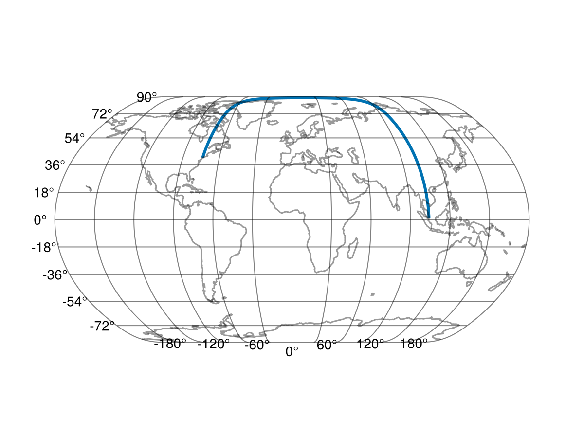

We'll use a satellite view for this, and alter the projection as a way of controlling the animation.

First, we'll create 2 observables which control the position of the "camera": distance along path (from 0 to 1) and altitude (in meters)!

The projection will always be centered at wherever the plane is.

We first create an animation through time, representing times (as hours), relative distances along the path, and altitudes of observation, as a function of time. This is done by using the Animations.jl library.

times = [0.0, 3.5, 14.5, 18]
distances = [0.0, 0.05, 0.95, 1]
altitudes = [357860.0*2, 35786000, 35786000, 357860*2]
distance_animation = Animation(times, distances, linear())
altitude_animation = Animation(times, altitudes, sineio())

Animations.Animation{Float64}(Animations.Keyframe{Float64}[Animations.Keyframe{Float64}(0.0, 715720.0), Animations.Keyframe{Float64}(3.5, 3.5786e7), Animations.Keyframe{Float64}(14.5, 3.5786e7), Animations.Keyframe{Float64}(18.0, 715720.0)], Animations.Easing[Animations.Easing{Animations.FuncEasing}(Animations.FuncEasing(Animations.f_sineio, ()), 1, false, 0.0, 0.0), Animations.Easing{Animations.FuncEasing}(Animations.FuncEasing(Animations.f_sineio, ()), 1, false, 0.0, 0.0), Animations.Easing{Animations.FuncEasing}(Animations.FuncEasing(Animations.f_sineio, ()), 1, false, 0.0, 0.0)])

In order to investigate this kind of projection, you can create a GeoAxis with the projection you want, and then change the altitude to see how the zoom works in real time!

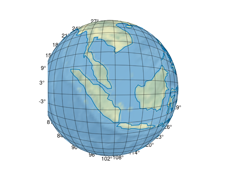
fig = Figure()
satview_projection = Observable("+proj=nsper +h=$(first(altitudes)) +lon_0=$(SIN[1]) +lat_0=$(SIN[2])")
ga = GeoAxis(fig[1, 1]; dest = satview_projection)
surface!(ga, -180..180, -90..90, zeros(axes(GeoMakie.earth() |> rotr90)); color = GeoMakie.earth() |> rotr90, shading = NoShading)
lines!(ga, GeoMakie.coastlines())
fig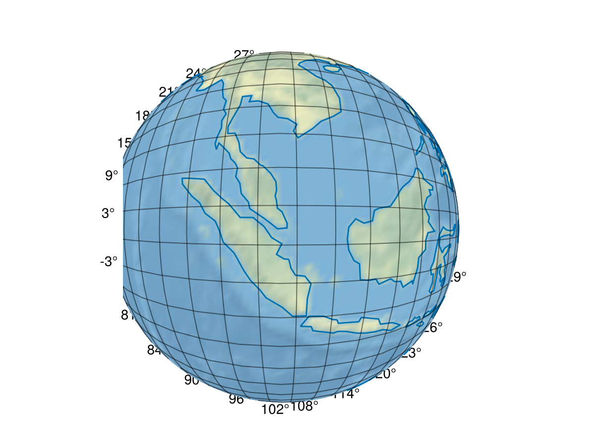

record(fig, "plane.mp4", LinRange(0, 1, 240)) do i
    current_position = Proj.geod_position_relative(inv_line, i)
    current_time = i * last(times)
    ga.dest[] = "+proj=nsper +h=$(round(Int, at(altitude_animation, current_time))) +lon_0=$(current_position[2]) +lat_0=$(current_position[1])"
end

"plane.mp4"

---

This page was generated using Literate.jl.