```@cardmeta
Title = "Raster warping, masking, plotting"
Description = "Semi involved example showing raster warping and masking, and plotting matrix lookup gridded data on a globe."
Cover = fig
```

`@cardmeta Title = 'Raster warping, masking, plotting' Description = 'Semi involved example showing raster warping and masking, and plotting matrix lookup gridded data on a globe.' Cover = fig`

In this example, we want to show how you can create manipulate rasters for the purpose of visualization.

using CairoMakie, GeoMakie
using Rasters, ArchGDAL,NaturalEarth, FileIO

Background setup

Set up the background. First, load the image,

blue_marble_image = FileIO.load(FileIO.query(download("https://eoimages.gsfc.nasa.gov/images/imagerecords/76000/76487/world.200406.3x5400x2700.jpg"))) |> rotr90 .|> RGBA{Makie.Colors.N0f8}

5400×2700 Array{RGBA{N0f8},2} with eltype RGBA{FixedPointNumbers.N0f8}:
 RGBA{N0f8}(0.929,0.929,0.929,1.0)  …  RGBA{N0f8}(0.043,0.055,0.114,1.0)
 RGBA{N0f8}(0.929,0.929,0.929,1.0)     RGBA{N0f8}(0.043,0.055,0.114,1.0)
 RGBA{N0f8}(0.929,0.929,0.929,1.0)     RGBA{N0f8}(0.047,0.059,0.118,1.0)
 RGBA{N0f8}(0.929,0.929,0.929,1.0)     RGBA{N0f8}(0.043,0.055,0.114,1.0)
 RGBA{N0f8}(0.929,0.929,0.929,1.0)     RGBA{N0f8}(0.039,0.051,0.11,1.0)
 RGBA{N0f8}(0.929,0.929,0.929,1.0)  …  RGBA{N0f8}(0.039,0.051,0.11,1.0)
 RGBA{N0f8}(0.929,0.929,0.929,1.0)     RGBA{N0f8}(0.039,0.051,0.11,1.0)
 RGBA{N0f8}(0.929,0.929,0.929,1.0)     RGBA{N0f8}(0.039,0.051,0.11,1.0)
 RGBA{N0f8}(0.918,0.918,0.918,1.0)     RGBA{N0f8}(0.039,0.051,0.11,1.0)
 RGBA{N0f8}(0.918,0.918,0.918,1.0)     RGBA{N0f8}(0.039,0.051,0.11,1.0)
 ⋮                                  ⋱  
 RGBA{N0f8}(0.925,0.925,0.925,1.0)     RGBA{N0f8}(0.49,0.502,0.522,1.0)
 RGBA{N0f8}(0.929,0.929,0.929,1.0)     RGBA{N0f8}(0.502,0.502,0.533,1.0)
 RGBA{N0f8}(0.929,0.929,0.929,1.0)     RGBA{N0f8}(0.502,0.502,0.533,1.0)
 RGBA{N0f8}(0.929,0.929,0.929,1.0)     RGBA{N0f8}(0.502,0.502,0.533,1.0)
 RGBA{N0f8}(0.929,0.929,0.929,1.0)  …  RGBA{N0f8}(0.502,0.502,0.533,1.0)
 RGBA{N0f8}(0.929,0.929,0.929,1.0)     RGBA{N0f8}(0.498,0.502,0.522,1.0)
 RGBA{N0f8}(0.929,0.929,0.929,1.0)     RGBA{N0f8}(0.498,0.502,0.522,1.0)
 RGBA{N0f8}(0.929,0.929,0.929,1.0)     RGBA{N0f8}(0.502,0.506,0.525,1.0)
 RGBA{N0f8}(0.929,0.929,0.929,1.0)     RGBA{N0f8}(0.506,0.51,0.529,1.0)

Your other choice is:

blue_marble_image = GeoMakie.earth() |> rotr90 .|> RGBA{Makie.Colors.N0f8}

720×360 Array{RGBA{N0f8},2} with eltype RGBA{FixedPointNumbers.N0f8}:
 RGBA{N0f8}(0.941,0.949,0.965,1.0)  …  RGBA{N0f8}(0.463,0.659,0.8,1.0)
 RGBA{N0f8}(0.941,0.949,0.965,1.0)     RGBA{N0f8}(0.463,0.659,0.8,1.0)
 RGBA{N0f8}(0.941,0.949,0.965,1.0)     RGBA{N0f8}(0.463,0.663,0.8,1.0)
 RGBA{N0f8}(0.941,0.949,0.965,1.0)     RGBA{N0f8}(0.463,0.663,0.8,1.0)
 RGBA{N0f8}(0.941,0.949,0.965,1.0)     RGBA{N0f8}(0.463,0.663,0.8,1.0)
 RGBA{N0f8}(0.941,0.949,0.965,1.0)  …  RGBA{N0f8}(0.463,0.663,0.8,1.0)
 RGBA{N0f8}(0.941,0.949,0.965,1.0)     RGBA{N0f8}(0.463,0.663,0.8,1.0)
 RGBA{N0f8}(0.941,0.953,0.965,1.0)     RGBA{N0f8}(0.467,0.663,0.8,1.0)
 RGBA{N0f8}(0.941,0.953,0.965,1.0)     RGBA{N0f8}(0.467,0.663,0.8,1.0)
 RGBA{N0f8}(0.945,0.953,0.965,1.0)     RGBA{N0f8}(0.467,0.663,0.8,1.0)
 ⋮                                  ⋱  
 RGBA{N0f8}(0.941,0.949,0.961,1.0)     RGBA{N0f8}(0.463,0.659,0.796,1.0)
 RGBA{N0f8}(0.941,0.949,0.961,1.0)     RGBA{N0f8}(0.463,0.659,0.8,1.0)
 RGBA{N0f8}(0.941,0.949,0.961,1.0)     RGBA{N0f8}(0.463,0.659,0.8,1.0)
 RGBA{N0f8}(0.941,0.949,0.961,1.0)     RGBA{N0f8}(0.463,0.659,0.8,1.0)
 RGBA{N0f8}(0.941,0.949,0.961,1.0)  …  RGBA{N0f8}(0.463,0.659,0.8,1.0)
 RGBA{N0f8}(0.941,0.949,0.961,1.0)     RGBA{N0f8}(0.463,0.659,0.8,1.0)
 RGBA{N0f8}(0.941,0.949,0.965,1.0)     RGBA{N0f8}(0.463,0.659,0.8,1.0)
 RGBA{N0f8}(0.941,0.949,0.965,1.0)     RGBA{N0f8}(0.463,0.659,0.796,1.0)
 RGBA{N0f8}(0.941,0.949,0.965,1.0)     RGBA{N0f8}(0.463,0.659,0.8,1.0)

For the purposes of this example, we'll use the Natural Earth background image, since it's significantly smaller and the poor CI machine can't handle huge images.

We wrap the image as a Raster for easy masking.

blue_marble_raster = Raster(
    blue_marble_image, # the contents
    ( # the dimensions go in this tuple.  `X` and `Y` are defined by the Rasters ecosystem.
        X(LinRange(-180, 180, size(blue_marble_image, 1))),
        Y(LinRange(-90, 90, size(blue_marble_image, 2)))
    )
)

╭────────────────────────────────────────────────╮
│ 720×360 Raster{RGBA{FixedPointNumbers.N0f8},2} │
├────────────────────────────────────────────────┴─────────────────────── dims ┐
  ↓ X Sampled{Float64} LinRange{Float64}(-180.0, 180.0, 720) ForwardOrdered Regular Points,
  → Y Sampled{Float64} LinRange{Float64}(-90.0, 90.0, 360) ForwardOrdered Regular Points
├────────────────────────────────────────────────────────────────────── raster ┤
  extent: Extent(X = (-180.0, 180.0), Y = (-90.0, 90.0))

└──────────────────────────────────────────────────────────────────────────────┘
    ↓ →    …  90.0
 -180.0         RGBA{N0f8}(0.463,0.659,0.8,1.0)
 -179.499       RGBA{N0f8}(0.463,0.659,0.8,1.0)
 -178.999       RGBA{N0f8}(0.463,0.663,0.8,1.0)
 -178.498       RGBA{N0f8}(0.463,0.663,0.8,1.0)
    ⋮      ⋱   ⋮
  177.997       RGBA{N0f8}(0.463,0.659,0.8,1.0)
  178.498       RGBA{N0f8}(0.463,0.659,0.8,1.0)
  178.999       RGBA{N0f8}(0.463,0.659,0.8,1.0)
  179.499       RGBA{N0f8}(0.463,0.659,0.796,1.0)
  180.0    …    RGBA{N0f8}(0.463,0.659,0.8,1.0)

Construct a mask of land using Natural Earth land polygons

land_mask = Rasters.boolmask(NaturalEarth.naturalearth("land", 10); to = blue_marble_raster)

╭────────────────────────╮
│ 720×360 Raster{Bool,2} │
├────────────────────────┴─────────────────────────────────────────────── dims ┐
  ↓ X Sampled{Float64} LinRange{Float64}(-180.0, 180.0, 720) ForwardOrdered Regular Points,
  → Y Sampled{Float64} LinRange{Float64}(-90.0, 90.0, 360) ForwardOrdered Regular Points
├────────────────────────────────────────────────────────────────────── raster ┤
  extent: Extent(X = (-180.0, 180.0), Y = (-90.0, 90.0))
  missingval: false
└──────────────────────────────────────────────────────────────────────────────┘
    ↓ →    -90.0  -89.4986  -88.9972  …  88.4958  88.9972  89.4986  90.0
 -180.0      0      1         1           0        0        0        0
 -179.499    0      1         1           0        0        0        0
 -178.999    0      1         1           0        0        0        0
 -178.498    0      1         1           0        0        0        0
    ⋮                                 ⋱                              ⋮
  177.997    0      1         1           0        0        0        0
  178.498    0      1         1           0        0        0        0
  178.999    0      1         1           0        0        0        0
  179.499    0      1         1           0        0        0        0
  180.0      0      0         0       …   0        0        0        0

Now, create a new raster as a copy of the background image, and set the values of all sea areas to be transparent.

land_raster = deepcopy(blue_marble_raster)
land_raster[(!).(land_mask)] .= RGBA{Makie.Colors.N0f8}(0.0, 0.0, 0.0, 0.0)
land_raster

╭────────────────────────────────────────────────╮
│ 720×360 Raster{RGBA{FixedPointNumbers.N0f8},2} │
├────────────────────────────────────────────────┴─────────────────────── dims ┐
  ↓ X Sampled{Float64} LinRange{Float64}(-180.0, 180.0, 720) ForwardOrdered Regular Points,
  → Y Sampled{Float64} LinRange{Float64}(-90.0, 90.0, 360) ForwardOrdered Regular Points
├────────────────────────────────────────────────────────────────────── raster ┤
  extent: Extent(X = (-180.0, 180.0), Y = (-90.0, 90.0))

└──────────────────────────────────────────────────────────────────────────────┘
    ↓ →    -90.0                           …  90.0
 -180.0       RGBA{N0f8}(0.0,0.0,0.0,0.0)       RGBA{N0f8}(0.0,0.0,0.0,0.0)
 -179.499     RGBA{N0f8}(0.0,0.0,0.0,0.0)       RGBA{N0f8}(0.0,0.0,0.0,0.0)
 -178.999     RGBA{N0f8}(0.0,0.0,0.0,0.0)       RGBA{N0f8}(0.0,0.0,0.0,0.0)
 -178.498     RGBA{N0f8}(0.0,0.0,0.0,0.0)       RGBA{N0f8}(0.0,0.0,0.0,0.0)
    ⋮                                      ⋱   ⋮
  177.997     RGBA{N0f8}(0.0,0.0,0.0,0.0)       RGBA{N0f8}(0.0,0.0,0.0,0.0)
  178.498     RGBA{N0f8}(0.0,0.0,0.0,0.0)       RGBA{N0f8}(0.0,0.0,0.0,0.0)
  178.999     RGBA{N0f8}(0.0,0.0,0.0,0.0)       RGBA{N0f8}(0.0,0.0,0.0,0.0)
  179.499     RGBA{N0f8}(0.0,0.0,0.0,0.0)       RGBA{N0f8}(0.0,0.0,0.0,0.0)
  180.0       RGBA{N0f8}(0.0,0.0,0.0,0.0)  …    RGBA{N0f8}(0.0,0.0,0.0,0.0)

Do the same for the sea.

sea_raster = deepcopy(blue_marble_raster)
sea_raster[land_mask] .= RGBA{Makie.Colors.N0f8}(0.0, 0.0, 0.0, 0.0)
sea_raster

╭────────────────────────────────────────────────╮
│ 720×360 Raster{RGBA{FixedPointNumbers.N0f8},2} │
├────────────────────────────────────────────────┴─────────────────────── dims ┐
  ↓ X Sampled{Float64} LinRange{Float64}(-180.0, 180.0, 720) ForwardOrdered Regular Points,
  → Y Sampled{Float64} LinRange{Float64}(-90.0, 90.0, 360) ForwardOrdered Regular Points
├────────────────────────────────────────────────────────────────────── raster ┤
  extent: Extent(X = (-180.0, 180.0), Y = (-90.0, 90.0))

└──────────────────────────────────────────────────────────────────────────────┘
    ↓ →    …  90.0
 -180.0         RGBA{N0f8}(0.463,0.659,0.8,1.0)
 -179.499       RGBA{N0f8}(0.463,0.659,0.8,1.0)
 -178.999       RGBA{N0f8}(0.463,0.663,0.8,1.0)
 -178.498       RGBA{N0f8}(0.463,0.663,0.8,1.0)
    ⋮      ⋱   ⋮
  177.997       RGBA{N0f8}(0.463,0.659,0.8,1.0)
  178.498       RGBA{N0f8}(0.463,0.659,0.8,1.0)
  178.999       RGBA{N0f8}(0.463,0.659,0.8,1.0)
  179.499       RGBA{N0f8}(0.463,0.659,0.796,1.0)
  180.0    …    RGBA{N0f8}(0.463,0.659,0.8,1.0)

Constructing fake data

Now, we construct fake data. First, we create a matrix of values.

field = [exp(cosd(x)) + 3(y/90) for x in -180:180, y in -90:90]

361×181 Matrix{Float64}:
 -2.63212  -2.59879  -2.56545  …  3.26788  3.30121  3.33455  3.36788
 -2.63206  -2.59873  -2.5654      3.26794  3.30127  3.3346   3.36794
 -2.6319   -2.59856  -2.56523     3.2681   3.30144  3.33477  3.3681
 -2.63162  -2.59828  -2.56495     3.26838  3.30172  3.33505  3.36838
 -2.63122  -2.59789  -2.56456     3.26878  3.30211  3.33544  3.36878
 -2.63072  -2.59738  -2.56405  …  3.26928  3.30262  3.33595  3.36928
 -2.6301   -2.59677  -2.56343     3.2699   3.30323  3.33657  3.3699
 -2.62937  -2.59603  -2.5627      3.27063  3.30397  3.3373   3.37063
 -2.62852  -2.59519  -2.56186     3.27148  3.30481  3.33814  3.37148
 -2.62756  -2.59423  -2.5609      3.27244  3.30577  3.3391   3.37244
  ⋮                            ⋱                             ⋮
 -2.62852  -2.59519  -2.56186     3.27148  3.30481  3.33814  3.37148
 -2.62937  -2.59603  -2.5627      3.27063  3.30397  3.3373   3.37063
 -2.6301   -2.59677  -2.56343     3.2699   3.30323  3.33657  3.3699
 -2.63072  -2.59738  -2.56405  …  3.26928  3.30262  3.33595  3.36928
 -2.63122  -2.59789  -2.56456     3.26878  3.30211  3.33544  3.36878
 -2.63162  -2.59828  -2.56495     3.26838  3.30172  3.33505  3.36838
 -2.6319   -2.59856  -2.56523     3.2681   3.30144  3.33477  3.3681
 -2.63206  -2.59873  -2.5654      3.26794  3.30127  3.3346   3.36794
 -2.63212  -2.59879  -2.56545  …  3.26788  3.30121  3.33455  3.36788

Then, we wrap it in a Raster. This is now gridded data, along the specified X and Y dimensions. Note the missingval = NaN keyword argument. This is used to indicate that if the raster does have missing values, they should be represented as NaN, and not 0, for example.

ras = Raster(field, (X(LinRange(-30, 30, size(field, 1))), Y(LinRange(-5, 5, size(field, 2)))); missingval = NaN)

╭───────────────────────────╮
│ 361×181 Raster{Float64,2} │
├───────────────────────────┴──────────────────────────────────────────── dims ┐
  ↓ X Sampled{Float64} LinRange{Float64}(-30.0, 30.0, 361) ForwardOrdered Regular Points,
  → Y Sampled{Float64} LinRange{Float64}(-5.0, 5.0, 181) ForwardOrdered Regular Points
├────────────────────────────────────────────────────────────────────── raster ┤
  extent: Extent(X = (-30.0, 30.0), Y = (-5.0, 5.0))
  missingval: NaN
└──────────────────────────────────────────────────────────────────────────────┘
   ↓ →     -5.0      -4.94444  …  4.83333  4.88889  4.94444  5.0
 -30.0     -2.63212  -2.59879     3.26788  3.30121  3.33455  3.36788
 -29.8333  -2.63206  -2.59873     3.26794  3.30127  3.3346   3.36794
 -29.6667  -2.6319   -2.59856     3.2681   3.30144  3.33477  3.3681
 -29.5     -2.63162  -2.59828     3.26838  3.30172  3.33505  3.36838
   ⋮                           ⋱                    ⋮        
  29.3333  -2.63122  -2.59789     3.26878  3.30211  3.33544  3.36878
  29.5     -2.63162  -2.59828     3.26838  3.30172  3.33505  3.36838
  29.6667  -2.6319   -2.59856     3.2681   3.30144  3.33477  3.3681
  29.8333  -2.63206  -2.59873  …  3.26794  3.30127  3.3346   3.36794
  30.0     -2.63212  -2.59879     3.26788  3.30121  3.33455  3.36788

We rotate the raster and then translate it to approximate the position in the image.

rotmat = Makie.rotmatrix2d(-π/5)

2×2 StaticArraysCore.SMatrix{2, 2, Float64, 4} with indices SOneTo(2)×SOneTo(2):
  0.809017  0.587785
 -0.587785  0.809017

We warp the raster by the parameters below. This is in total basically rotating the raster by the rotation matrix rotmat, and then translating it by 30 units in the x direction and -36 in the y direction.

This is where the missingval keyword argument comes in. If we didn't have it, the values that are now NaN because they are outside the original raster would be filled by 0, which is not what we want.

Rasters.warp is pretty much a wrapper around GDAL's gdalwarp program, so all of the options are available. It's incredibly versatile and flexible but is a bit tricky to use.

transformed = Rasters.warp(
    ras,
    Dict(
        "r" => "bilinear",
        "ct" => #= see https://gdal.org/en/latest/programs/gdalwarp.html =# """
        +proj=pipeline
        +step +proj=affine +xoff=$(30) +yoff=$(-36) +s11=$(rotmat[1,1]) +s12=$(rotmat[1,2]) +s21=$(rotmat[2,1]) +s22=$(rotmat[2,2])
        """,
        "s_srs" => "+proj=longlat +datum=WGS84 +type=crs",
        "t_srs" => "+proj=longlat +datum=WGS84 +type=crs",
    )
)

╭───────────────────────────╮
│ 361×288 Raster{Float64,2} │
├───────────────────────────┴──────────────────────────────────────────── dims ┐
  ↓ X Projected{Float64} LinRange{Float64}(2.7823459563862345, 57.16214601458978, 361) ForwardOrdered Regular Points,
  → Y Projected{Float64} LinRange{Float64}(-57.678215207187165, -14.32543016078601, 288) ForwardOrdered Regular Points
├──────────────────────────────────────────────────────────────────── metadata ┤
  Metadata{Rasters.GDALsource} of Dict{String, Any} with 4 entries:
  "units"    => ""
  "offset"   => 0.0
  "filepath" => "/vsimem/tmp"
  "scale"    => 1.0
├────────────────────────────────────────────────────────────────────── raster ┤
  extent: Extent(X = (2.7823459563862345, 57.16214601458978), Y = (-57.678215207187165, -14.32543016078601))
  missingval: NaN
  crs: GEOGCS["unknown",DATUM["WGS_1984",SPHEROID["WGS 84",6378137,298.257223563,AUTHORITY["EPSG","7030"]],AUTHORITY["EPSG","6326"]],PRIMEM["Greenwich",0,AUTHORITY["EPSG","8901"]],UNIT["degree",0.0174532925199433,AUTHORITY["EPSG","9122"]],AXIS["Longitude",EAST],AXIS["Latitude",NORTH]]
└──────────────────────────────────────────────────────────────────────────────┘
  ↓ →      -57.6782  -57.5272  -57.3761  …  -14.6275  -14.4765  -14.3254
  2.78235  NaN       NaN       NaN          NaN       NaN       NaN
  ⋮                                      ⋱                      
 57.1621   NaN       NaN       NaN          NaN       NaN       NaN

Plotting the data

We use an orthographic GeoAxis to show the data. First, we create the figure and the axis,

fig = Figure()
ax = GeoAxis(fig[1, 1]; dest = "+proj=ortho +lon_0=0 +lat_0=0")

GeoAxis()

Then, we plot the sea and land rasters. These are our background images.

sea_plot = meshimage!(ax, sea_raster; source = "+proj=longlat +datum=WGS84 +type=crs", npoints = 300)

land_plot = meshimage!(ax, land_raster; source = "+proj=longlat +datum=WGS84 +type=crs", npoints = 300)

Plot{GeoMakie.meshimage, Tuple{MakieCore.EndPoints{Float64}, MakieCore.EndPoints{Float64}, Matrix{RGBA{FixedPointNumbers.N0f8}}}}

Finally, we plot the transformed data.

data_plot = surface!(ax, transformed; shading = NoShading)

Surface{Tuple{Vector{Float64}, Vector{Float64}, Matrix{Float32}}}

Get the land plot above all other plots in the geoaxis.

translate!(land_plot, 0, 0, 1)

3-element Vec{3, Float64} with indices SOneTo(3):
 0.0
 0.0
 1.0

Display the figure...

fig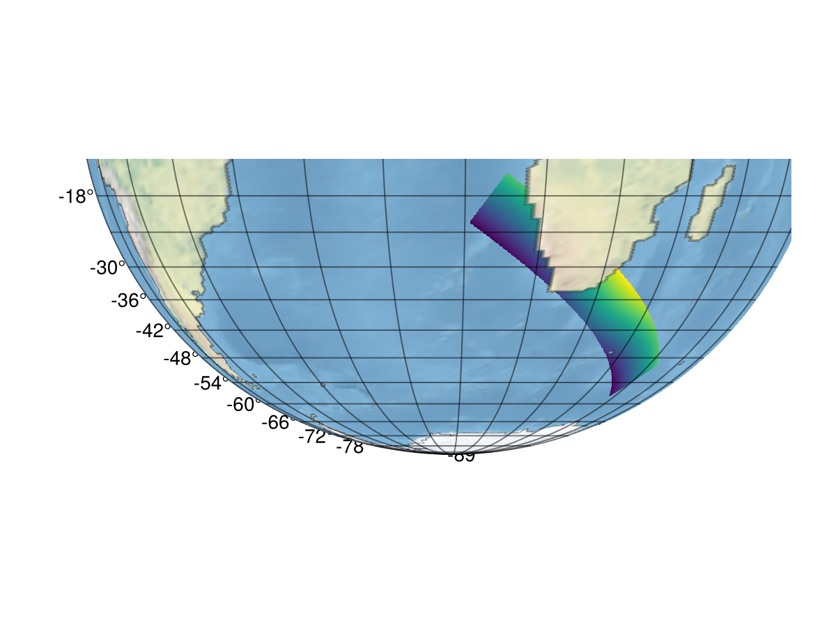

For extra credit, we'll find the center of the raster and transform the orthographic projection to be centered on it:

using Statistics
xy_matrix = Rasters.DimensionalData.DimPoints(transformed) |> collect
center_x = mean(first.(xy_matrix))
center_y = mean(last.(xy_matrix))

-36.00182268398659

We'll use the ortho projection, which is centered on the point we just found.

ax.dest[] = "+proj=ortho +lon_0=$(center_x) +lat_0=$(center_y)"

"+proj=ortho +lon_0=29.972245985488005 +lat_0=-36.00182268398659"

Somehow, the limits are set to the wrong thing, so we'll set them manually and let the axis take care of it.

ax.limits[] = (-180, 180, -90, 90)
fig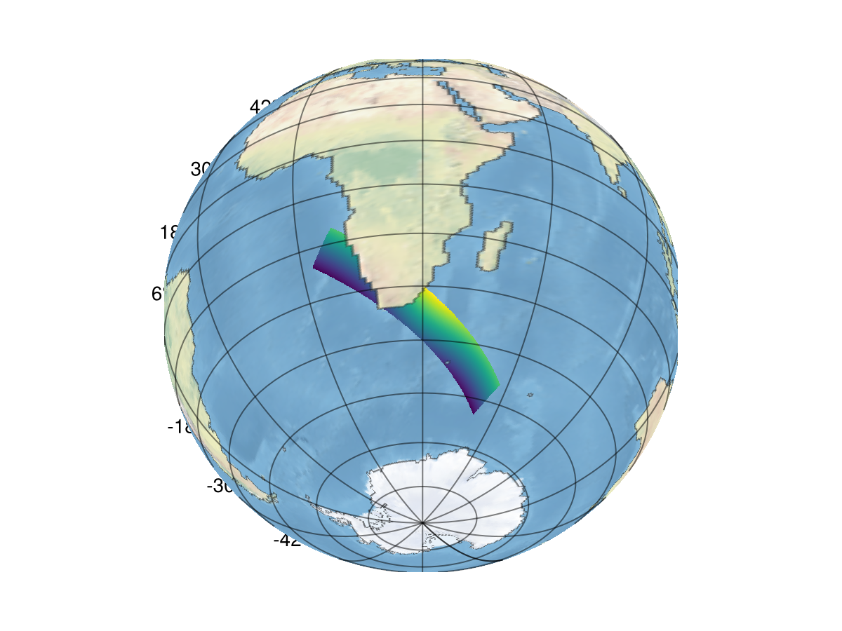

Plotting on the 3D globe

Super bonus points: plot the data on the globe

using Geodesy

fig = Figure(size = (1000, 1000));

fig2 = Figure()

ax = LScene(fig2[1, 1])

sea_plot = meshimage!(ax, sea_raster; npoints = 300)

land_plot = meshimage!(ax, land_raster; npoints = 300)

data_plot = surface!(ax, transformed; shading = NoShading)

land_plot.z_level[] = 1000 # this means raising land by 1 km over the sea!

sea_plot.transformation.transform_func[] = Geodesy.ECEFfromLLA(Geodesy.WGS84())
land_plot.transformation.transform_func[] = Geodesy.ECEFfromLLA(Geodesy.WGS84())
data_plot.transformation.transform_func[] = Geodesy.ECEFfromLLA(Geodesy.WGS84())

fig2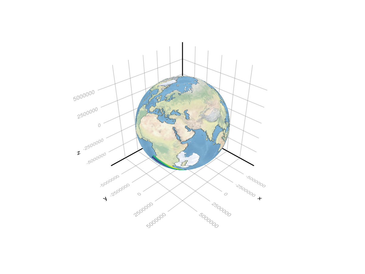

---

This page was generated using Literate.jl.