Histogram

You can use any Makie compatible recipe in GeoMakie, and this includes histograms! Until we get the datashader recipe working, you can also consider this a replacement for that if you use it with the correct nbins.

We use the excellent FHist.jl to create the histogram.

using CairoMakie, GeoMakie
using FHist
import CairoMakie: Point2d

First, we generate random points in a normal distribution:

random_data = randn(Point2d, 100_000)

100000-element Vector{GeometryBasics.Point{2, Float64}}:
 [0.6754862951293035, 1.4906617231853074]
 [0.6520008887923876, -1.040531908576004]
 [-0.39172910645925135, 0.4744958685157418]
 [0.17519910381362191, -0.9911943300274848]
 [0.595822951280291, 1.2653631136597427]
 [2.323013384963523, 0.9175325988649834]
 [-0.09962376593188846, 1.913179339132747]
 [1.154189030339875, 2.0920385702842696]
 [0.09965891988433616, -1.215898873872802]
 [-2.4033668599983455, 0.404265342870232]
 ⋮
 [-0.17986242051506254, -0.9867224541946011]
 [0.3402341966191378, 0.3873308126379098]
 [0.9030596077813113, 0.47996681597157487]
 [0.7789891858261573, 0.9271884753324315]
 [-0.5912588440153376, 0.5825896515006439]
 [-1.1042123046480228, -0.707959501213339]
 [-0.3793185874567793, 1.2702325399419316]
 [0.4852458393946008, -0.9467797505826502]
 [1.6472218064878505, 0.20638199484346914]

then, we rescale them to be within the lat/long bounds of the Earth:

xmin, xmax = extrema(first, random_data)
ymin, ymax = extrema(last, random_data)
latlong_data = random_data .* (Point2d(1/(xmax - xmin), 1/(ymax - ymin)) * Point2d(360, 180),)

100000-element Vector{GeometryBasics.Point{2, Float64}}:
 [28.365060579020085, 30.943079534256878]
 [27.37886000282334, -21.599307947747505]
 [-16.449511878187096, 9.849560882790371]
 [7.356971161216723, -20.57516102473384]
 [25.019832717998867, 26.26634256229641]
 [97.54811587665375, 19.046094590317196]
 [-4.183407089298835, 39.71367851827665]
 [48.466774235536604, 43.426429257680724]
 [4.184883276155565, -25.23956641179711]
 [-100.92232376737228, 8.391719236371758]
 ⋮
 [-7.552793432799893, -20.4823340557361]
 [14.287134569190181, 8.040193127058167]
 [37.921332624934536, 9.963126529254977]
 [32.711360105582585, 19.24653077839262]
 [-24.828176454958374, 12.093366081540172]
 [-46.36814860536139, -14.695786986645485]
 [-15.928368627967913, 26.367421863114572]
 [20.37647207558897, -19.65320546441706]
 [69.17023582124168, 4.284066855378824]

finally, we can create the histogram.

h = Hist2D((first.(latlong_data), last.(latlong_data)); nbins = (360, 180))

• edges: ([-190.0, -189.0, -188.0, -187.0, -186.0, -185.0, -184.0, -183.0, -182.0, -181.0 … 162.0, 163.0, 164.0, 165.0, 166.0, 167.0, 168.0, 169.0, 170.0, 171.0], [-89.0, -88.0, -87.0, -86.0, -85.0, -84.0, -83.0, -82.0, -81.0, -80.0 … 83.0, 84.0, 85.0, 86.0, 87.0, 88.0, 89.0, 90.0, 91.0, 92.0])
• bin counts: [0.0 0.0 … 0.0 0.0; 0.0 0.0 … 0.0 0.0; … ; 0.0 0.0 … 0.0 0.0; 0.0 0.0 … 0.0 0.0]
• maximum count: 33.0
• total count: 100000.0

This is what the histogram looks like without any projection,

plot(h)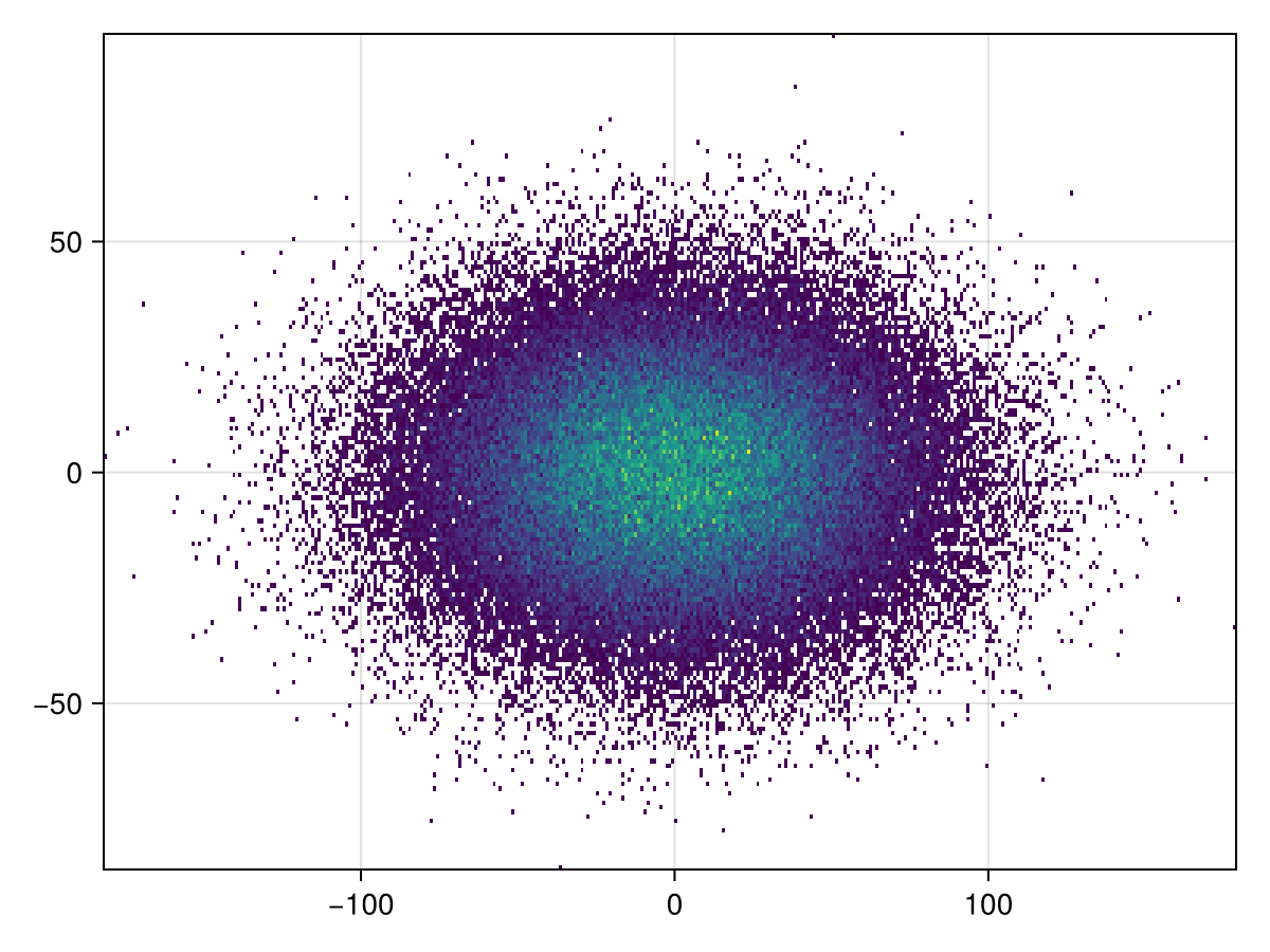

It's simple to plot to GeoAxis:

plot(h; axis = (; type = GeoAxis))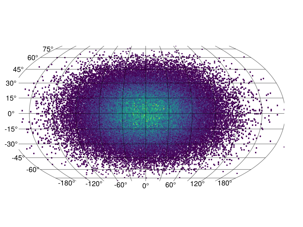

The projection can also be arbitrary!

plot(h; axis = (; type = GeoAxis, dest = "+proj=tissot +lat_1=60 +lat_2=65"))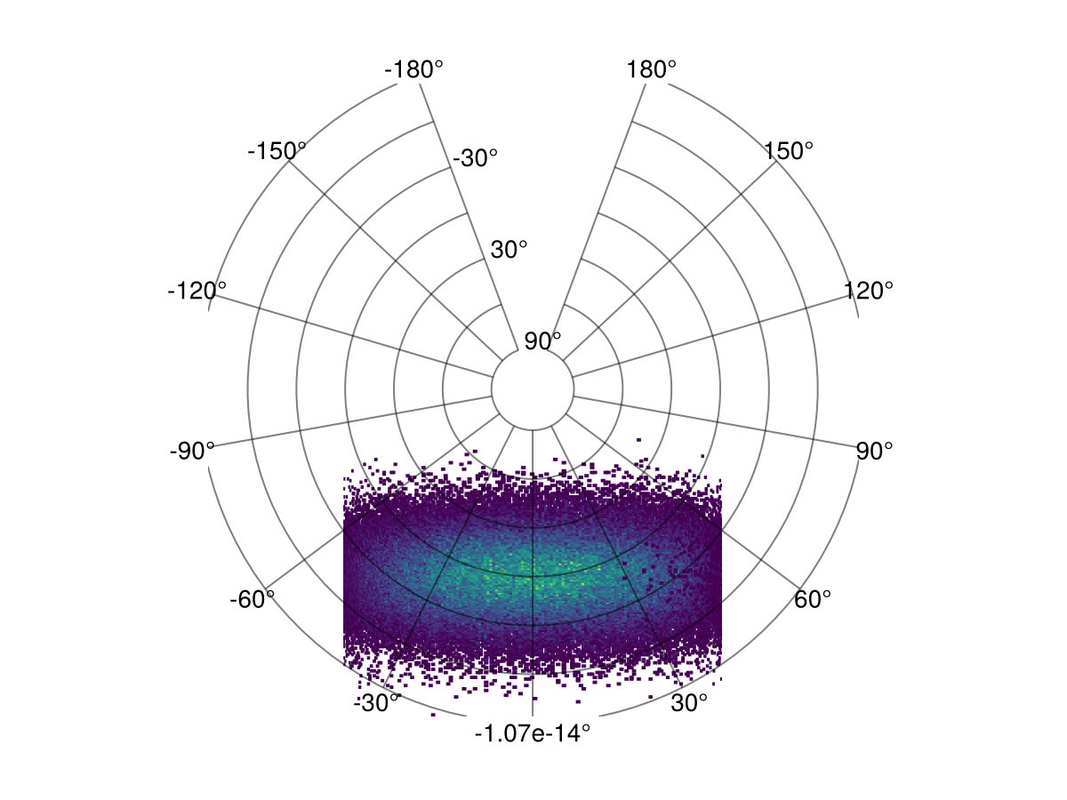

---

This page was generated using Literate.jl.