Contours

using Makie, GeoMakie, CairoMakie

lons = -180:180
lats = -90:90

-90:90

Create some field of values across lons and lats.

This grid can be of any density, but note that the time it takes to plot scales with the grid size!

field = [exp(cosd(l)) + 3(y/90) for l in lons, y in lats]

361×181 Matrix{Float64}:
 -2.63212  -2.59879  -2.56545  …  3.26788  3.30121  3.33455  3.36788
 -2.63206  -2.59873  -2.5654      3.26794  3.30127  3.3346   3.36794
 -2.6319   -2.59856  -2.56523     3.2681   3.30144  3.33477  3.3681
 -2.63162  -2.59828  -2.56495     3.26838  3.30172  3.33505  3.36838
 -2.63122  -2.59789  -2.56456     3.26878  3.30211  3.33544  3.36878
 -2.63072  -2.59738  -2.56405  …  3.26928  3.30262  3.33595  3.36928
 -2.6301   -2.59677  -2.56343     3.2699   3.30323  3.33657  3.3699
 -2.62937  -2.59603  -2.5627      3.27063  3.30397  3.3373   3.37063
 -2.62852  -2.59519  -2.56186     3.27148  3.30481  3.33814  3.37148
 -2.62756  -2.59423  -2.5609      3.27244  3.30577  3.3391   3.37244
  ⋮                            ⋱                             ⋮
 -2.62852  -2.59519  -2.56186     3.27148  3.30481  3.33814  3.37148
 -2.62937  -2.59603  -2.5627      3.27063  3.30397  3.3373   3.37063
 -2.6301   -2.59677  -2.56343     3.2699   3.30323  3.33657  3.3699
 -2.63072  -2.59738  -2.56405  …  3.26928  3.30262  3.33595  3.36928
 -2.63122  -2.59789  -2.56456     3.26878  3.30211  3.33544  3.36878
 -2.63162  -2.59828  -2.56495     3.26838  3.30172  3.33505  3.36838
 -2.6319   -2.59856  -2.56523     3.2681   3.30144  3.33477  3.3681
 -2.63206  -2.59873  -2.5654      3.26794  3.30127  3.3346   3.36794
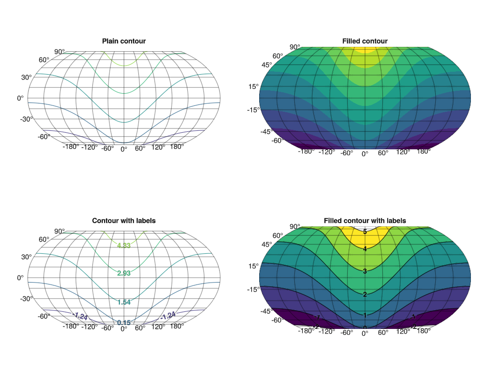
 -2.63212  -2.59879  -2.56545  …  3.26788  3.30121  3.33455  3.36788

Makie provides two main recipes for contours = contour for lines, and contourf for fills. In this example, we'll see examples of both.

Regular contour

fig = Figure(size = (1000, 750), Contour = (; labelsize = 14, labelfont = :bold), Text = (; strokecolor = :gray, strokewidth = .3))
ax1 = GeoAxis(fig[1,1]; title = "Plain contour")
contour!(ax1, lons, lats, field)
fig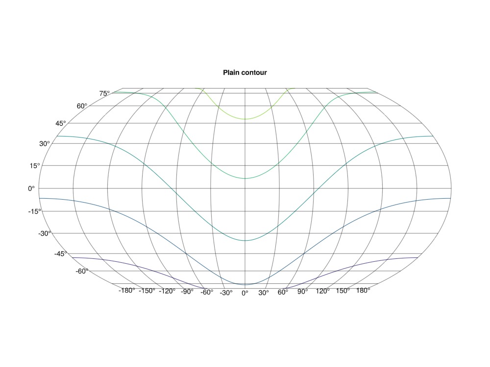

Filled contour

Makie also offers filled contours via the contourf recipe:

ax2 = GeoAxis(fig[1,2]; title = "Filled contour")
contourf!(ax2, lons, lats, field)
fig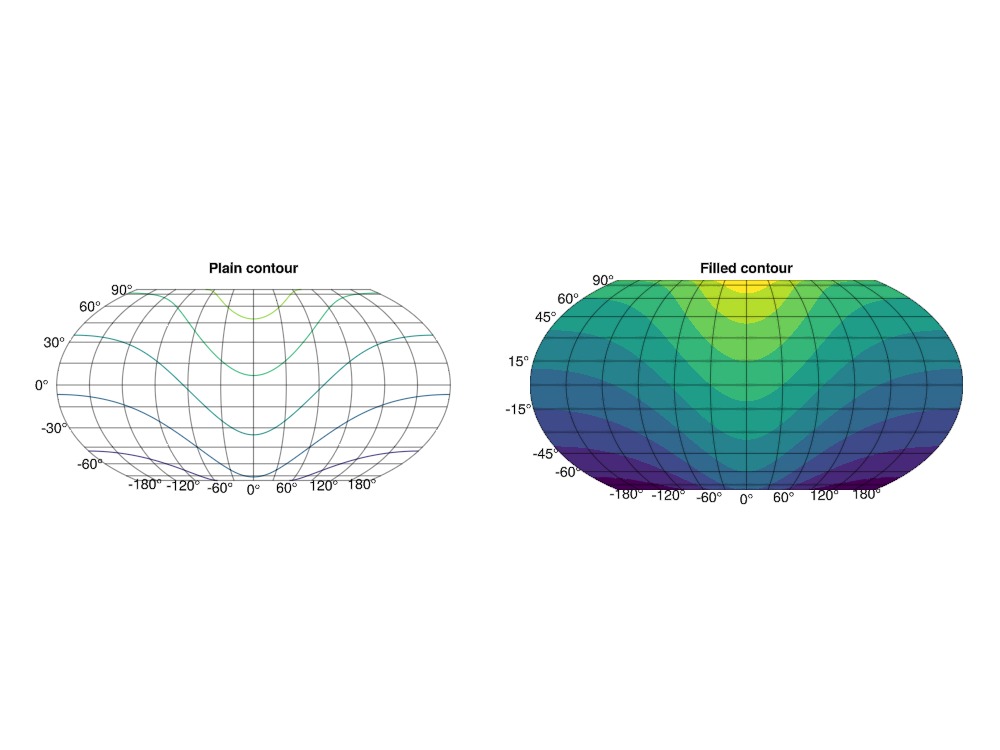

Contour with labels

The contour recipe also offers labels, which we can activate via keyword:

ax3 = GeoAxis(fig[2,1]; title = "Contour with labels")
contour!(ax3, lons, lats, field; labels = true)
fig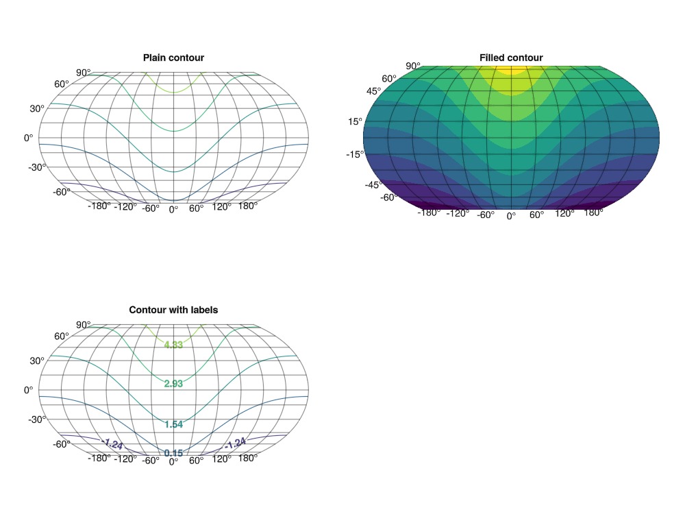

Filled contour with labels

Finally, we can get a filled contour plot with labels by connecting the levels from the contourf plot to the contour plot:

ax4 = GeoAxis(fig[2,2]; title = "Filled contour with labels")
cfp = contourf!(ax4, lons, lats, field)
clp = contour!(
    ax4, lons, lats, field;
    color = :black, labels = true,
    levels = cfp.computed_levels
)
fig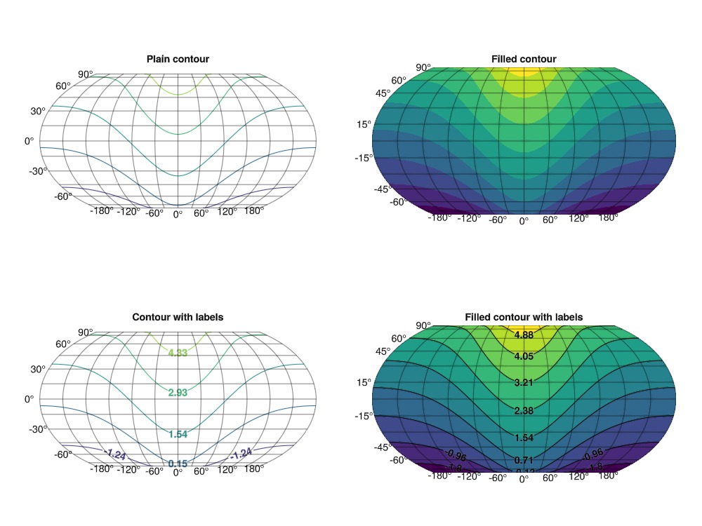

In order to control the levels, we need only set the levels for the first filled contour plot:

cfp.levels[] = -2:5
fig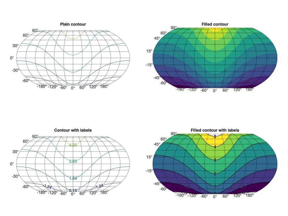

---

This page was generated using Literate.jl.