GeoMakie.jl

GeoMakie.jl is a Julia package for plotting geospatial data on a given map projection. It is based on the Makie.jl plotting ecosystem.

The package ClimateBase.jl builds upon GeoMakie.jl to create a seamless workflow between analyzing/manipulating climate data, and plotting them.

Installation

This package is in development and may break, although we are currently working on a long-term stable interface.

You can install it from the REPL like so:

]add GeoMakie

GeoAxis

Using GeoMakie.jl is straightforward, although it does assume basic knowledge of the Makie.jl ecosystem.

GeoMakie.jl provides an axis for plotting geospatial data, GeoAxis. Both are showcased in the examples below.

Gotchas

When plotting a projection which has a limited domain (in either longitude or latitude), if your limits are not inside that domain, the axis will appear blank. To fix this, simply correct the limits - you can even do it on the fly, using the xlims!(ax, low, high) or ylims!(ax, low, high) functions.

Useful data sources

• NaturalEarth.jl provides access to all of the Natural Earth datasets, like coastlines, land polygons, country borders, rivers, and so on.

• GADM.jl provides access to the GADM cultural data, including the borders of all countries and their sub-divisions,from the GADM dataset (https://gadm.org/)..

• GeoDatasets.jl provides access to the GSHHG dataset.

• RasterDataSources.jl

Examples

Surface example

using GeoMakie, CairoMakie

lons = -180:180
lats = -90:90
field = [exp(cosd(l)) + 3(y/90) for l in lons, y in lats]

fig = Figure()
ax = GeoAxis(fig[1,1])
surface!(ax, lons, lats, field; shading = NoShading)
fig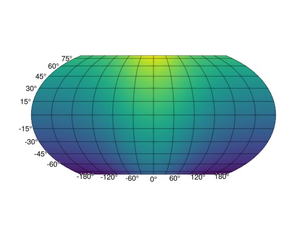

Scatter example

using GeoMakie, CairoMakie

lons = -180:180
lats = -90:90
slons = rand(lons, 2000)
slats = rand(lats, 2000)
sfield = [exp(cosd(l)) + 3(y/90) for (l,y) in zip(slons, slats)]

fig = Figure()
ax = GeoAxis(fig[1,1])
scatter!(slons, slats; color = sfield)
fig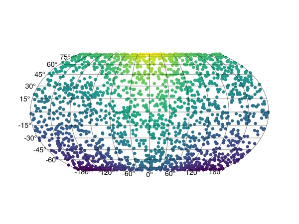

Map projections

The default projection is given by the arguments source = "+proj=longlat +datum=WGS84", dest = "+proj=eqearth", so that if a different one is needed, for example a wintri projection one can do it as follows:

using GeoMakie, CairoMakie

lons = -180:180
lats = -90:90
field = [exp(cosd(l)) + 3(y/90) for l in lons, y in lats]

fig = Figure()
ax = GeoAxis(fig[1,1]; dest = "+proj=wintri")
surface!(ax, lons, lats, field; shading = NoShading)
fig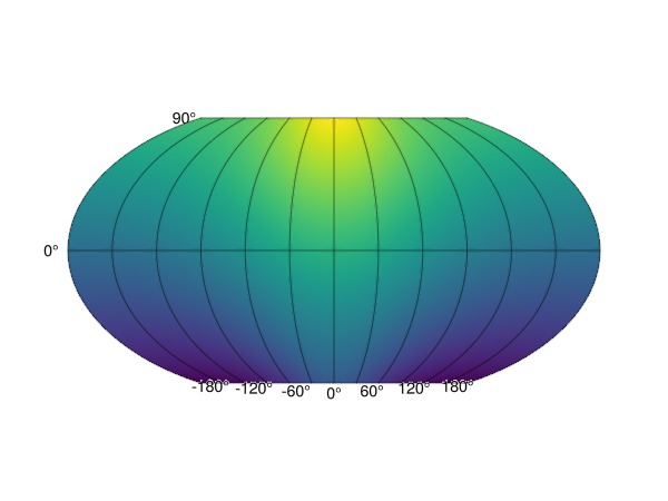

Changing central longitude

Be careful! Each data point is transformed individually. However, when using surface or contour plots this can lead to errors when the longitudinal dimension "wraps" around the planet.

E.g., if the data have the dimensions

lons = 0.5:359.5
lats = -90:90
field = [exp(cosd(l)) + 3(y/90) for l in lons, y in lats];

360×181 Matrix{Float64}:
 -0.281822  -0.248488  -0.215155  …  5.61818  5.65151  5.68484  5.71818
 -0.282649  -0.249316  -0.215983     5.61735  5.65068  5.68402  5.71735
 -0.284304  -0.250971  -0.217637     5.6157   5.64903  5.68236  5.7157
 -0.286784  -0.25345   -0.220117     5.61322  5.64655  5.67988  5.71322
 -0.290085  -0.256751  -0.223418     5.60992  5.64325  5.67658  5.70992
 -0.294204  -0.260871  -0.227537  …  5.6058   5.63913  5.67246  5.7058
 -0.299136  -0.265802  -0.232469     5.60086  5.6342   5.66753  5.70086
 -0.304874  -0.271541  -0.238208     5.59513  5.62846  5.66179  5.69513
 -0.311413  -0.278079  -0.244746     5.58859  5.62192  5.65525  5.68859
 -0.318743  -0.28541   -0.252077     5.58126  5.61459  5.64792  5.68126
  ⋮                               ⋱                             ⋮
 -0.311413  -0.278079  -0.244746     5.58859  5.62192  5.65525  5.68859
 -0.304874  -0.271541  -0.238208     5.59513  5.62846  5.66179  5.69513
 -0.299136  -0.265802  -0.232469     5.60086  5.6342   5.66753  5.70086
 -0.294204  -0.260871  -0.227537     5.6058   5.63913  5.67246  5.7058
 -0.290085  -0.256751  -0.223418  …  5.60992  5.64325  5.67658  5.70992
 -0.286784  -0.25345   -0.220117     5.61322  5.64655  5.67988  5.71322
 -0.284304  -0.250971  -0.217637     5.6157   5.64903  5.68236  5.7157
 -0.282649  -0.249316  -0.215983     5.61735  5.65068  5.68402  5.71735
 -0.281822  -0.248488  -0.215155     5.61818  5.65151  5.68484  5.71818

a surface! plot with the default arguments will lead to artifacts if the data along longitude 179 and 180 have significantly different values. To fix this, there are two approaches: (1) to change the central longitude of the map transformation, by changing the projection destination used like so:

ax = GeoAxis(fig[1,1]; dest = "+proj=eqearth +lon_0=180")

or (2), circshift your data appropriately so that the central longitude you want coincides with the center of the longitude dimension of the data.

Countries loaded with GeoJSON

using GeoMakie, CairoMakie

# First, make a surface plot
lons = -180:180
lats = -90:90
field = [exp(cosd(l)) + 3(y/90) for l in lons, y in lats]

fig = Figure()
ax = GeoAxis(fig[1,1])
sf = surface!(ax, lons, lats, field; shading = NoShading)
cb1 = Colorbar(fig[1,2], sf; label = "field", height = Relative(0.65))

using NaturalEarth
countries = naturalearth("admin_0_countries", 110)

n = length(countries)
hm = poly!(ax, GeoMakie.to_multipoly(countries.geometry); color= 1:n, colormap = :dense,
    strokecolor = :black, strokewidth = 0.5,
)
translate!(hm, 0, 0, 100) # move above surface plot

fig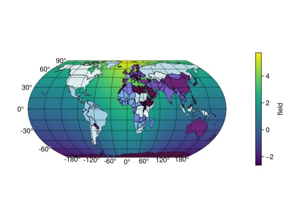

Gotchas

With CairoMakie, we recommend that you use image!(ga, ...) or heatmap!(ga, ...) to plot images or scalar fields into ga::GeoAxis.

However, with GLMakie, which is much faster, these methods do not work; if you have used them, you will see an empty axis. If you want to plot an image img, you can use a surface in the following way: surface!(ga, lonmin..lonmax, latmin..latmax, ones(size(img)...); color = img, shading = NoShading).

To plot a scalar field, simply use surface!(ga, lonmin..lonmax, latmin..latmax, field). The .. notation denotes an interval which Makie will automatically sample from to obtain the x and y points for the surface.

API

GeoMakie.to_multipoly Function

to_multipoly(geom)

Convert a polygon, vector of polygons, multipolygon, or any GeoInterface-compatible geometry into a GeometryBasics.MultiPolygon. GeometryCollections are handled by extracting their polygon and multipolygon members and unioning them.

source

GeoMakie.geo2basic Function

geo2basic(input)

Takes any GeoInterface-compatible structure, and returns its equivalent in the GeometryBasics.jl package, which Makie is built on.

Currently works for the following traits:

- PointTrait
- LineTrait
- LineStringTrait
- PolygonTrait
- MultiPolygonTrait

source

GeoMakie.geoformat_ticklabels Function

geoformat_ticklabels(nums::Vector)

A semi-intelligent formatter for geographic tick labels. Append "ᵒ" to the end of each tick label, to indicate degree.

This will check whether the ticklabel is an integer value (round(num) == num). If so, label as an Int (1 instead of 1.0) which looks a lot cleaner.

Example

julia> geoformat_ticklabels([1.0, 1.1, 2.5, 25])
4-element Vector{String}:
 "1ᵒ"
 "1.1ᵒ"
 "2.5ᵒ"
 "25ᵒ"

source

GeoAxis, meshimage, and the rest of the public API are documented on the API reference page.