Satellite dashboard

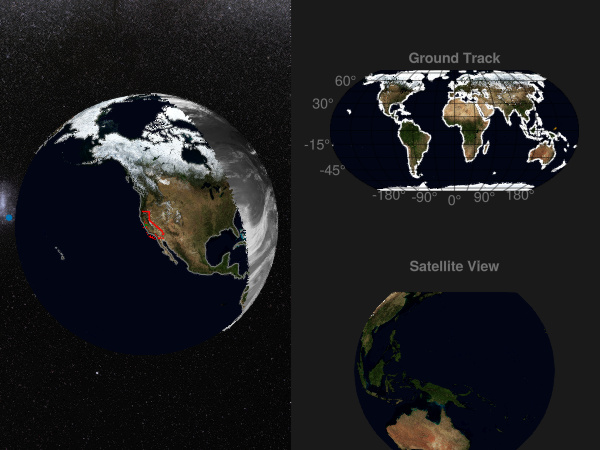
In this example, we'll build a live dashboard that shows the orbit of a satellite, along with a ground track and a "simulation" of the view from the satellite.

To simulate the satellite's trajectory, we'll use the SatelliteToolbox.jl ecosystem.

The dashboard's visuals will come from GeoMakieArtifacts.jl, which exposes the NASA Blue Marble images and full-sky map from the European Southern Observatory.

using GeoMakie, GLMakie
using GeoMakieArtifacts

using Geodesy, Proj
import GeometryOps as GO, GeoInterface as GI
using SatelliteToolbox

Utility functions

Utility functions

From gadomski/antimeridian on github

function crossing_latitude_flat(p1, p2)
    latitude_delta = p2[2] - p1[2]
    return if p2[1] > 0
        p1[2] + (180 - p1[1]) * latitude_delta / (p2[1] + 360 - p1[1])
    else
        p1[2] + (p1[1] + 180) * latitude_delta / (p1[1] + 360 - p2[1])
    end
end

const proj_transf_from_cart_to_longlat = GeoMakie.create_transform("+proj=longlat +datum=WGS84", "+proj=cart +type=crs")

function splitify(pos, color)
    newpos = Tuple{Float64, Float64}[]
    sizehint!(newpos, length(pos))
    newcolor = similar(color, 0)
    sizehint!(newcolor, length(color))

    p1 = proj_transf_from_cart_to_longlat(pos[1])[1:2]
    p2 = p1
    push!(newpos, p1)
    push!(newcolor, color[1])
    for i in 2:length(pos)
        p2 = proj_transf_from_cart_to_longlat(pos[i])[1:2]

        needs_split, sign = if p2[1] - p1[1] > 180 && p2[1] - p1[1] != 360
            true, -1
        elseif p1[1] - p2[1] > 180 && p1[1] - p2[1] != 360
            true, 1
        else
            false, 0
        end

        if needs_split
            crossing_latitude = sign == -1 ? crossing_latitude_flat(p1, p2) : crossing_latitude_flat(p2, p1)
            push!(newpos, (sign * 180.0, crossing_latitude))
            push!(newcolor, color[i])
            push!(newpos, (NaN, NaN))
            push!(newcolor, color[i])
            push!(newpos, (-sign * 180.0, crossing_latitude))
            push!(newcolor, color[i])
        end
        push!(newpos, p2)
        push!(newcolor, color[i])
        p1 = p2
    end
    return (newpos, newcolor)
end

splitify (generic function with 1 method)

Data acquisition

Background images and attribution

First, get some data - we have a skymap and a globe image.

skymap_image = joinpath(geomakie_artifact_dir("skymap"), "skymap.png") |> Makie.FileIO.load
skymap_attrib = get_attribution("skymap")

globe_image = joinpath(geomakie_artifact_dir("blue_marble_topo_november"), "image.png") |> Makie.FileIO.load
globe_attrib = get_attribution("blue_marble_topo_november")

"NASA/Visible Earth"

Geospatial data

Let's get some geometries of interest that we can plot on the globe. For now, let's take the state of California and the county of Santa Clara. We'll use the GADM.jl package to get these.

using GADM
cali = GADM.get("USA", "California")
sc_county = GADM.get("USA", "California", "Santa Clara")

GADM.Table{Vector{Any}, GeoFormatTypes.WellKnownText{GeoFormatTypes.CRS}}(Any[Feature
  (index 0) geom => MULTIPOLYGON
  (index 0) GID_2 => USA.5.43_1
  (index 1) GID_0 => USA
  (index 2) COUNTRY => United States
  (index 3) GID_1 => USA.5_1
  (index 4) NAME_1 => California
  (index 5) NL_NAME_1 => NA
  (index 6) NAME_2 => Santa Clara
  (index 7) VARNAME_2 => NA
  (index 8) NL_NAME_2 => NA
  (index 9) TYPE_2 => County
...
 Number of Fields: 13], GeoFormatTypes.WellKnownText{GeoFormatTypes.CRS}(GeoFormatTypes.CRS(), "GEOGCS[\"WGS 84\",DATUM[\"WGS_1984\",SPHEROID[\"WGS 84\",6378137,298.257223563,AUTHORITY[\"EPSG\",\"7030\"]],AUTHORITY[\"EPSG\",\"6326\"]],PRIMEM[\"Greenwich\",0,AUTHORITY[\"EPSG\",\"8901\"]],UNIT[\"degree\",0.0174532925199433,AUTHORITY[\"EPSG\",\"9122\"]],AXIS[\"Latitude\",NORTH],AXIS[\"Longitude\",EAST],AUTHORITY[\"EPSG\",\"4326\"]]"))

Satellite trajectory

Let's take the Hubble Space Telescope as an example here. We can get the TLE and simulate its orbit from SatelliteToolbox.jl. But, any data source will do, so long as it provides position and velocity vectors in an earth-centered, earth-fixed frame.

tle = SatelliteToolbox.tle"""
HST
1 20580U 90037B   25298.18540833  .00010258  00000+0  36633-3 0  9991
2 20580  28.4680 242.7474 0002152  56.7096 303.3705 15.27131570752566
"""

prop = SatelliteToolbox.Propagators.init(Val(:SGP4), tle)
sv_teme = SatelliteToolbox.Propagators.propagate!(prop, 0:1:(86400 * 30), OrbitStateVector)
eop = SatelliteToolbox.fetch_iers_eop()
sv_itrf = SatelliteToolbox.sv_eci_to_ecef.(sv_teme, (TEME(),), (SatelliteToolbox.ITRF(),), (eop,))

2592001-element Vector{SatelliteToolboxBase.OrbitStateVector{Float64, Float64}}:
 OrbitStateVector{Float64, Float64}: Epoch = 2.46097e6 (2025-10-25T04:26:59.280)
 OrbitStateVector{Float64, Float64}: Epoch = 2.46097e6 (2025-10-25T04:27:00.280)
 OrbitStateVector{Float64, Float64}: Epoch = 2.46097e6 (2025-10-25T04:27:01.280)
 OrbitStateVector{Float64, Float64}: Epoch = 2.46097e6 (2025-10-25T04:27:02.280)
 OrbitStateVector{Float64, Float64}: Epoch = 2.46097e6 (2025-10-25T04:27:03.280)
 OrbitStateVector{Float64, Float64}: Epoch = 2.46097e6 (2025-10-25T04:27:04.280)
 OrbitStateVector{Float64, Float64}: Epoch = 2.46097e6 (2025-10-25T04:27:05.280)
 OrbitStateVector{Float64, Float64}: Epoch = 2.46097e6 (2025-10-25T04:27:06.280)
 OrbitStateVector{Float64, Float64}: Epoch = 2.46097e6 (2025-10-25T04:27:07.280)
 OrbitStateVector{Float64, Float64}: Epoch = 2.46097e6 (2025-10-25T04:27:08.280)
 ⋮
 OrbitStateVector{Float64, Float64}: Epoch = 2.461e6 (2025-11-24T04:26:51.280)
 OrbitStateVector{Float64, Float64}: Epoch = 2.461e6 (2025-11-24T04:26:52.280)
 OrbitStateVector{Float64, Float64}: Epoch = 2.461e6 (2025-11-24T04:26:53.280)
 OrbitStateVector{Float64, Float64}: Epoch = 2.461e6 (2025-11-24T04:26:54.280)
 OrbitStateVector{Float64, Float64}: Epoch = 2.461e6 (2025-11-24T04:26:55.280)
 OrbitStateVector{Float64, Float64}: Epoch = 2.461e6 (2025-11-24T04:26:56.280)
 OrbitStateVector{Float64, Float64}: Epoch = 2.461e6 (2025-11-24T04:26:57.280)
 OrbitStateVector{Float64, Float64}: Epoch = 2.461e6 (2025-11-24T04:26:58.280)
 OrbitStateVector{Float64, Float64}: Epoch = 2.461e6 (2025-11-24T04:26:59.280)

Plotting!

Background imagery and orbit lines

First, let's create a Figure and place a GlobeAxis in it. We'll also add some background imagery: the NASA Blue Marble earth image, and a full-sky map from the European Southern Observatory.

A couple things to note here:

• The uv_transform keyword is used to rotate the image so that it looks like it's on the globe.

• The zlevel keyword is used to control the depth of the image.

• The xautolimits, yautolimits, and zautolimits keywords are used to control the limits of the axis.

• The reset_limits keyword is used to reset the limits of the axis when the camera is moved.

f = with_theme(theme_dark()) do
    Figure(; figure_padding = 0)
end
a = GlobeAxis(f[1, 1]; show_axis = false)
sky_plot = meshimage!(a, -180..180, -90..90, skymap_image; uv_transform = :rotr90, zlevel = 7e7, xautolimits = false, yautolimits = false, zautolimits = false, reset_limits = false)
globe_plot = meshimage!(a, -180..180, -90..90, globe_image; uv_transform = :rotr90, zlevel = 0, reset_limits = false)
f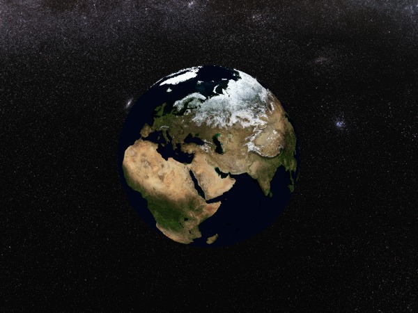

Camera positioning

It's possible to directly position the camera in ECEF space, which requires a little bit of manual transformation. First, we'll get the centroid of the Santa Clara county, which we want the camera to hover over.

sc_centroid = GO.centroid(sc_county)

(-121.69289129108222, 37.231239081227585)

Then, we'll update the GeoAxis camera to look at the centroid.

Makie.update_cam!(a; longlat = sc_centroid)
f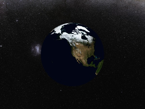

Note that to display the figure faithfully with these exact camera settings, you should run display(f; update = false) to avoid automatically updating the camera. Similary to save, run save("dashboard.png", f; update = false).

Satellite orbit lines

Now, let's plot the satellite orbit lines. This is a simple line plot, but it's already in ECEF space! So we can just indicate via the source keyword that it doesn't need to be transformed.

But that's not all - you can plot any data from any projection, and it will get transformed appropriately. So a satellite image, for example, can go directly onto the globe in its native projection, and will look correct.

orbit_plot = lines!(
    a,
    getproperty.(sv_itrf[1:86400÷2], :r); # get the position from the state vector
    transparency = false,
    color = :lightblue,
    source = "+proj=cart +type=crs",
)
f
# Let's also plot some coastlines just for a visual reference.
coastline_plot = lines!(a, GeoMakie.coastlines(); color = :gray, linewidth = 1, zlevel = 20_000)
f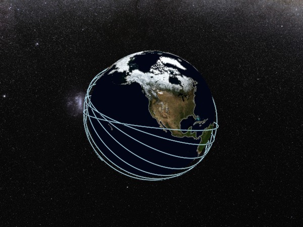

Areas of interest

You can use any "sensible" plot recipe on a GlobeAxis, it will get transformed correctly to the globe. Let's plot some 3D bands to highlight areas of interest - in this case, California and the Santa Clara county.

cali_lower, cali_upper = GeoMakie.geom_to_bands(cali; height = 25_000)
sc_lower, sc_upper = GeoMakie.geom_to_bands(sc_county; height = 40_000)
cali_band_plot = band!(a, cali_lower, cali_upper; color = :red)
lines!(a, cali_lower; color = :red)
sc_band_plot = band!(a, sc_lower, sc_upper; color = :green)
lines!(a, sc_lower; color = :green)
f

Images

You can also easily overlay an image, or a series of images, with any colormap, transparency, et cetera. It's as simple as getting the data and then plotting it, with either the meshimage! or surface! recipes. To begin, let's plot a real satellite image

using Downloads, FileIO
geostationary_img = FileIO.load(Downloads.download("https://gist.github.com/pelson/5871263/raw/EIDA50_201211061300_clip2.png"))
mi = meshimage!(a,
    -5500000 .. 5500000, -5500000 .. 5500000, geostationary_img;
    source="+proj=geos +h=35786000",
    npoints=1000,
    zlevel = 100_000,
)

Plot{GeoMakie.meshimage, Tuple{Makie.EndPoints{Float64}, Makie.EndPoints{Float64}, IndirectArrays.IndirectArray{RGB{FixedPointNumbers.N0f8}, 2, UInt8, Matrix{UInt8}, OffsetArrays.OffsetVector{RGB{FixedPointNumbers.N0f8}, Vector{RGB{FixedPointNumbers.N0f8}}}}}}

Animating the plot

Let's do an animation of the plot, by showing the satellite orbit over time. We'll add a play button and a text field to control the speedup, and let the last 90 minutes of the orbit be visible at any point.

orbit_plot.visible[] = false

satellite_graph = Makie.ComputeGraph()

Makie.add_input!(satellite_graph, :time_rel, 0.001)

Makie.map!(satellite_graph, [:time_rel], [:satellite_position, :satellite_trajectory]) do t
    pos = sv_itrf[round(Int, t * 86400) + 1].r
    traj = getproperty.(view(sv_itrf, max(1, round(Int, t * 86400) - 180 * 30):round(Int, t * 86400) + 1), :r)
    return (pos, traj)
end
Makie.map!(satellite_graph, [:satellite_trajectory], [:satellite_trajectory_color]) do traj
    color = if length(traj) == 1
        RGBAf[Makie.wong_colors(1.0)[2]]
    else
        RGBAf.((Makie.wong_colors()[2],), LinRange(0, 1, length(traj)))
    end
    return (color,)
end

satellite_marker_plt = scatter!(
    a.scene, satellite_graph[:satellite_position];
)

satellite_trajectory_plt = lines!(
    a.scene,
    satellite_graph[:satellite_trajectory];
    color = satellite_graph[:satellite_trajectory_color]
)

Lines{Tuple{Vector{Point{3, Float64}}}}

Trace of satellite path on GeoAxis

We can also plot the trace of the satellite path on a GeoAxis off to the side.

diag_gl = GridLayout(f[1, 2]; alignmode = Outside())
ground_ax = GeoAxis(diag_gl[1, 1]; limits = ((-180, 180), (-90, 90)), title = "Ground Track")
meshimage!(ground_ax, -180..180, -90..90, globe_image; uv_transform = :rotr90)
lines!(ground_ax, GeoMakie.coastlines(); color = :white)
satellite_marker_ground_plt = scatter!(
    ground_ax,
    satellite_graph[:satellite_position];
    source = "+proj=cart +type=crs",
    marker = :circle,
    color = :blue,
    strokecolor = :white,
    strokewidth = 1
)

map!(
    splitify,
    satellite_graph,
    [:satellite_trajectory, :satellite_trajectory_color],
    [:satellite_trajectory_cut, :satellite_position_color_cut]
)

ComputeGraph():
  Inputs:
    :time_rel => Input(:time_rel, 0.001)

  Outputs:
    :satellite_position           => Computed(:satellite_position, [-5.723373871068188e6, 3.7680613604206424e6, 312397.4650246087])
    :satellite_position_color_cut => Computed(:satellite_position_color_cut, #undef)
    :satellite_trajectory         => Computed(:satellite_trajectory, StaticArraysCore.SVector{3, Float64}[[-5.419014448500881e6, 4.206362021788922e6, 21.12016504473209], [-5.4228114370039925e6, 4.201455550230643e6, 3658.961798812813], [-5.42660246507305e6, 4.1965444594048e6, 7296.798894499123], [-5.430387528771266e6, 4.1916287543819584e6, 10934.626941436907], [-5.434166611718793e6, 4.186708456396242e6, 14572.441428905586], [-5.437939734614443e6, 4.1817835385992024e6, 18210.237846176813], [-5.441706881113519e6, 4.176854022177036e6, 21848.01168255652], [-5.445468047160447e6, 4.1719199124093824e6, 25485.758427335448], [-5.449223228923356e6, 4.1669812142978064e6, 29123.473569828577], [-5.452972422323741e6, 4.162037933179374e6, 32761.152599360976]  …  [-5.693658025716215e6, 3.8154324144253307e6, 279791.7883255771], [-5.696984808252819e6, 3.8101857531076046e6, 283416.08914926986], [-5.700305352455587e6, 3.8049348680674946e6, 287040.0384953549], [-5.703619643555659e6, 3.7996797816810776e6, 290663.6318689149], [-5.706927678234665e6, 3.7944204992502904e6, 294286.8647754236], [-5.710229452818864e6, 3.78915702662575e6, 297909.7327207995], [-5.713524964003381e6, 3.7838893691185927e6, 301532.2312113937], [-5.716814208227263e6, 3.778617532440558e6, 305154.35575399565], [-5.720097182100563e6, 3.7733415220605065e6, 308776.10185583023], [-5.723373871068188e6, 3.7680613604206424e6, 312397.4650246087]])
    :satellite_trajectory_color   => Computed(:satellite_trajectory_color, RGBA{Float32}[RGBA(0.9019608, 0.62352943, 0.0, 0.0), RGBA(0.9019608, 0.62352943, 0.0, 0.011627907), RGBA(0.9019608, 0.62352943, 0.0, 0.023255814), RGBA(0.9019608, 0.62352943, 0.0, 0.034883723), RGBA(0.9019608, 0.62352943, 0.0, 0.046511628), RGBA(0.9019608, 0.62352943, 0.0, 0.058139537), RGBA(0.9019608, 0.62352943, 0.0, 0.069767445), RGBA(0.9019608, 0.62352943, 0.0, 0.08139535), RGBA(0.9019608, 0.62352943, 0.0, 0.093023255), RGBA(0.9019608, 0.62352943, 0.0, 0.10465116)  …  RGBA(0.9019608, 0.62352943, 0.0, 0.89534885), RGBA(0.9019608, 0.62352943, 0.0, 0.90697676), RGBA(0.9019608, 0.62352943, 0.0, 0.9186047), RGBA(0.9019608, 0.62352943, 0.0, 0.9302326), RGBA(0.9019608, 0.62352943, 0.0, 0.94186044), RGBA(0.9019608, 0.62352943, 0.0, 0.95348835), RGBA(0.9019608, 0.62352943, 0.0, 0.96511626), RGBA(0.9019608, 0.62352943, 0.0, 0.9767442), RGBA(0.9019608, 0.62352943, 0.0, 0.9883721), RGBA(0.9019608, 0.62352943, 0.0, 1.0)])
    :satellite_trajectory_cut     => Computed(:satellite_trajectory_cut, #undef)
    :time_rel                     => Computed(:time_rel, 0.001)

satellite_trajectory_ground_plt = lines!(
    ground_ax,
    satellite_graph[:satellite_trajectory_cut];
    color = satellite_graph[:satellite_position_color_cut]
)

view_label = Label(
    diag_gl[2, 1], "Satellite View";
    halign = :center, font = :bold,
    tellheight = true, tellwidth = false
)
view_ax = GlobeAxis(diag_gl[3, 1]; show_axis = false, center = false)
meshimage!(view_ax, -180..180, -90..90, globe_image; uv_transform = :rotr90)
f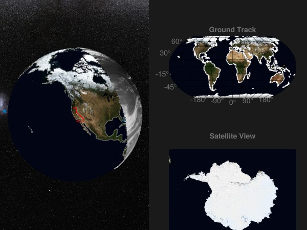

Extract camera controls for the view axis. We'll use this to update the camera to be at the satellite's predicted position.

cc = Makie.cameracontrols(view_ax.scene)
# Update the camera when the satellite position changes
cam_controller = on(view_ax.scene, satellite_graph.satellite_position; update = true) do ecef
    time_rel = satellite_graph.time_rel[]
    lookat = Vec3d(0,0,0)
    eyeposition = ecef .* 2    ## TODO: some coordinate system shenanigans here
    upvector = Makie.normalize(sv_itrf[round(Int, time_rel * 86400) + 1].v)
    Makie.update_cam!(view_ax.scene, eyeposition, lookat, upvector)
    return nothing
end

f

Animation: Play button and dynamic speedup

Here's the dashboard controls to run the animation interactively.

controls_gl = GridLayout(diag_gl[4, 1]; alignmode = Outside())
play_button = Button(controls_gl[1, 1]; tellwidth = false, tellheight = true, label = "▶")
is_playing = Observable(false)

timestep_field = Textbox(controls_gl[1, 2]; placeholder = "0.001 days/frame", validator = Float64, tellwidth = false, tellheight = false)
timestep = Observable(0.001)
colgap!(controls_gl, 1, 0)

on(timestep_field.stored_string) do stored_string
    timestep[] = parse(Float64, stored_string)
end

play_button_text_listener = on(play_button.clicks; priority = 1000) do _
    is_playing[] = !is_playing[]
    if is_playing[]
        play_button.label[] = "||"
    else
        play_button.label[] = "▶"
    end
end
player_listener = Makie.Observables.on(events(f).tick) do tick
    tr = satellite_graph.time_rel
    if is_playing[]
        tic = time()
        if tr[] > 30 - 52 * timestep[]
            tr[] = 0.001
        else
            tr[] += timestep[]
        end
        yield()
        toc = time()
    else
        ## do nothing
    end
end
satellite_graph.time_rel[] = 1
f

---

This page was generated using Literate.jl.