Histogram

You can use any Makie compatible recipe in GeoMakie, and this includes histograms! Until we get the datashader recipe working, you can also consider this a replacement for that if you use it with the correct nbins.

We use the excellent FHist.jl to create the histogram.

using GLMakie, GeoMakie
using FHist
import GLMakie: Point2d

First, we generate random points in a normal distribution:

random_data = randn(Point2d, 100_000)

100000-element Vector{Point{2, Float64}}:
 [0.06806287526108952, -0.4028711788593605]
 [-0.9462123796584875, 0.43973932532234367]
 [0.604581799360701, 0.7426816733409972]
 [-2.1558661777884844, -0.05110889736925235]
 [-0.5898269315379626, 0.038201426327174076]
 [-1.088194775428943, 0.8525955856314772]
 [2.589546103157154, 1.501006513416506]
 [0.0012244886674615501, -0.1303220819794289]
 [-0.8841436933192603, -0.532709740156697]
 [-0.4613094333951765, 0.3172302505228295]
 ⋮
 [0.8809659258153726, 1.3926241229381464]
 [1.3646374728587194, 0.809572612686098]
 [0.904730446010765, -1.4925624882776005]
 [-0.7079969349415006, 0.38901013239299365]
 [-0.0829628932203921, 1.449791946657217]
 [1.6349744934921269, -0.3957103416445168]
 [-1.4809644779444286, -1.5695279542572453]
 [-0.22654221521787082, -0.14930851724764418]
 [0.7311707191543497, 0.4653079636569187]

then, we rescale them to be within the lat/long bounds of the Earth:

xmin, xmax = extrema(first, random_data)
ymin, ymax = extrema(last, random_data)
latlong_data = random_data .* (Point2d(1/(xmax - xmin), 1/(ymax - ymin)) * Point2d(360, 180),)

100000-element Vector{Point{2, Float64}}:
 [2.9172548575808213, -8.09779405083547]
 [-40.55577508697866, 8.838851422917918]
 [25.913086748456085, 14.928055298154582]
 [-92.4029591068877, -1.0272994117704586]
 [-25.28067576576206, 0.7678565732139669]
 [-46.641307503343015, 17.137347676849693]
 [110.99099060076595, 30.170541484310654]
 [0.052483023961331435, -2.6195008119801915]
 [-37.89543821416533, -10.707575997063117]
 [-19.77226469286823, 6.376393671798466]
 ⋮
 [37.75923536273689, 27.992033010917545]
 [58.48996653848074, 16.27257701901128]
 [38.77781063908463, -30.000814831913896]
 [-30.345581048222133, 7.819184148951962]
 [-3.5558871457860537, 29.14111809593701]
 [70.07692908746945, -7.953859741209401]
 [-63.475878746161435, -31.547836622587386]
 [-9.709865697802352, -3.0011320892456195]
 [31.33883668580922, 9.352786343703018]

finally, we can create the histogram.

h = Hist2D((first.(latlong_data), last.(latlong_data)); nbins = (360, 180))

• edges: ([-180.0, -179.0, -178.0, -177.0, -176.0, -175.0, -174.0, -173.0, -172.0, -171.0 … 172.0, 173.0, 174.0, 175.0, 176.0, 177.0, 178.0, 179.0, 180.0, 181.0], [-86.0, -85.0, -84.0, -83.0, -82.0, -81.0, -80.0, -79.0, -78.0, -77.0 … 86.0, 87.0, 88.0, 89.0, 90.0, 91.0, 92.0, 93.0, 94.0, 95.0])
• bin counts: [0.0 0.0 … 0.0 0.0; 0.0 0.0 … 0.0 0.0; … ; 0.0 0.0 … 0.0 0.0; 0.0 0.0 … 0.0 0.0]
• maximum count: 32.0
• total count: 100000.0

This is what the histogram looks like without any projection,

plot(h)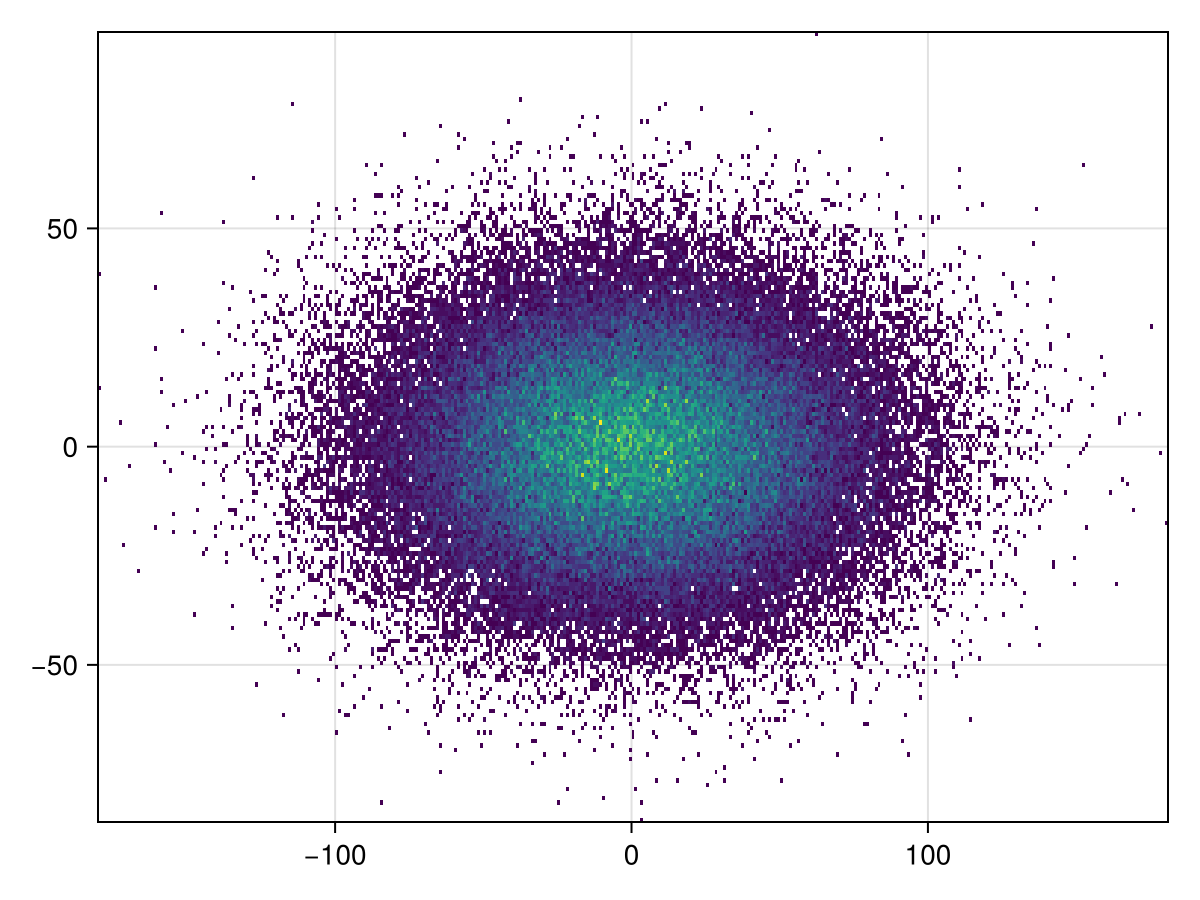

It's simple to plot to GeoAxis:

plot(h; axis = (; type = GeoAxis))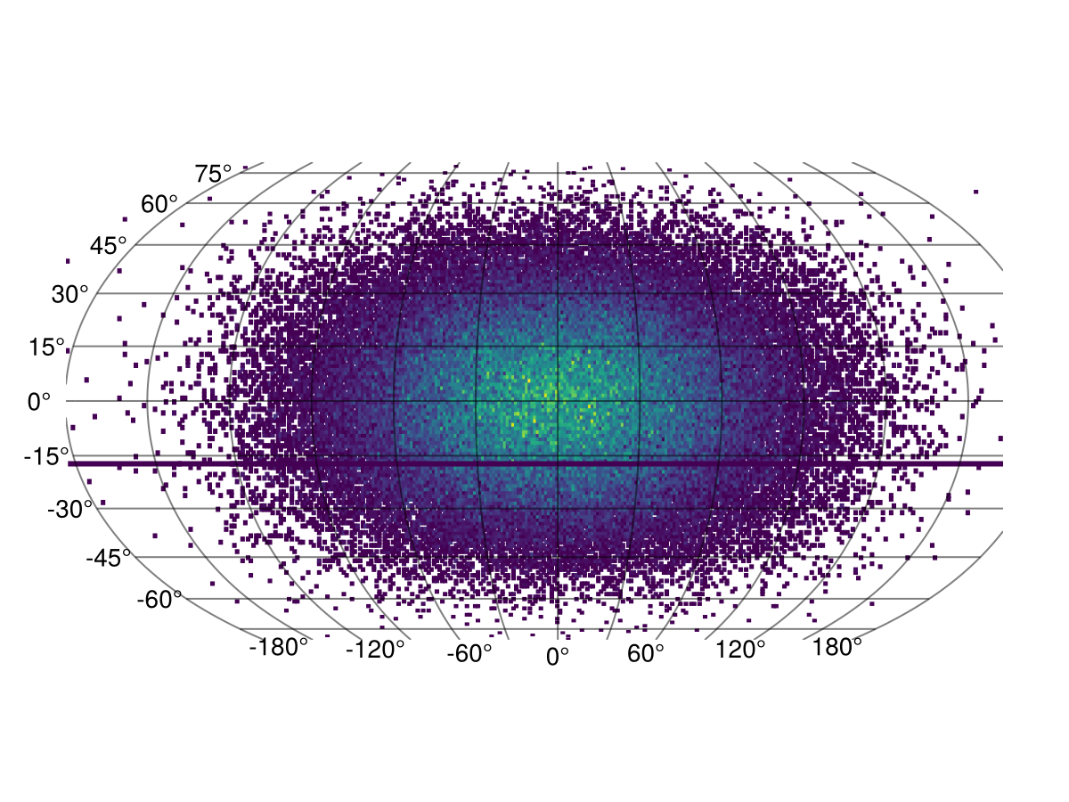

The projection can also be arbitrary!

plot(h; axis = (; type = GeoAxis, dest = "+proj=tissot +lat_1=60 +lat_2=65"))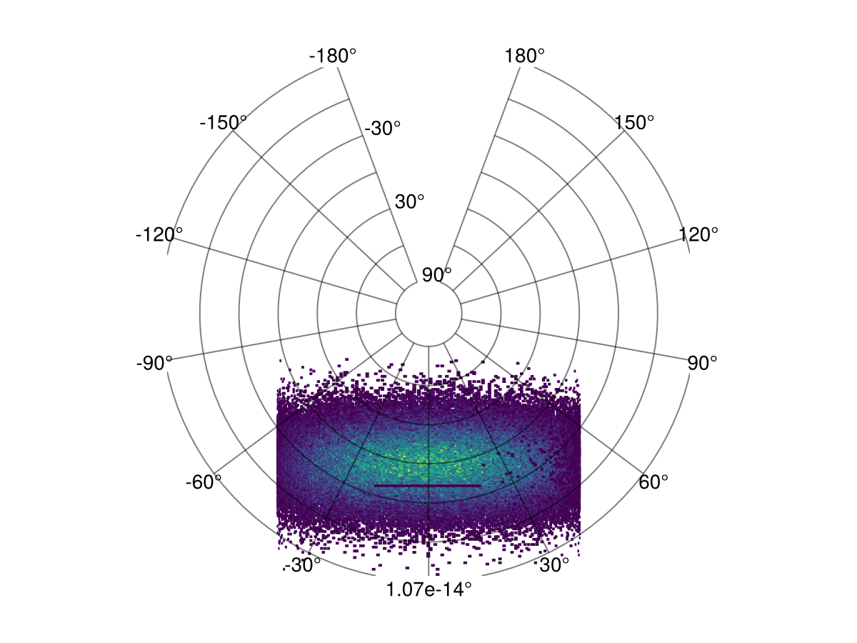

---

This page was generated using Literate.jl.