Pure Julia code
Fast, understandable, extensible functions
GeoMakie.jl is a Julia package for plotting geospatial data on a given map projection. It is built on top of the Makie.jl plotting ecosystem.
GeoMakie provides a GeoAxis type which handles CRS and projections, and various utilities and integrations to handle plotting geometries. GeoAxis should work seamlessly with any Makie plotting function, and can be used as a drop-in replacement for Makie.Axis.
The main entry point to GeoMakie is the function GeoAxis(fig[i, j]; kw_args...). It creates an axis which accepts nonlinear projections, but is otherwise identical in usage to Makie's Axis. Projections are accepted as PROJ-strings, and can be set through the source="+proj=latlong +datum=WGS84" and dest="+proj=eqearth" keyword arguments to GeoAxis.
using CairoMakie, GeoMakie

fig = Figure()
ga = GeoAxis(
    fig[1, 1]; # any cell of the figure's layout
    dest = "+proj=wintri", # the CRS in which you want to plot
)
lines!(ga, GeoMakie.coastlines()) # plot coastlines from Natural Earth as a reference
# You can plot your data the same way you would in Makie
scatter!(ga, -120:15:120, -60:7.5:60; color = -60:7.5:60, strokecolor = (:black, 0.2))
fig
As you can see, the axis automatically transforms your input from the source CRS (default "+proj=longlat +datum=WGS84") to the dest CRS.
Be careful! Each data point is transformed individually. However, when using surface or contour plots this can lead to errors when the longitudinal dimension "wraps" around the planet.
To fix this issue, the recommended approach is that you (1) change the central longitude of the map transformation (dest), and (2) circshift your data accordingly for lons and field.
function cshift(lons, field, lon_0)
   shift = @. lons - lon_0 > 180
   nn = sum(shift)
   (circshift(lons - 360shift, nn), circshift(field, (nn, 0)))
end
cshift (generic function with 1 method)lons = -180:180
lats = -90:90
field = [exp(cosd(l)) + 3(y/90) for l in lons, y in lats]
lon_0 = -160
(lons_shift, field_shift) = cshift(lons, field, lon_0)([-339, -338, -337, -336, -335, -334, -333, -332, -331, -330 … 11, 12, 13, 14, 15, 16, 17, 18, 19, 20], [-0.4563999336474307 -0.4230666003140975 … 5.510266733019236 5.543600066352569; -0.47261832807133697 -0.43928499473800375 … 5.49404833859533 5.527381671928663; … ; -0.42585207717080964 -0.3925187438374764 … 5.540814589495858 5.574147922829191; -0.4408053458235157 -0.4074720124901825 … 5.525861320843151 5.559194654176484])fig = Figure()
ax = GeoAxis(fig[1,1]; dest = "+proj=eqearth +lon_0=$(lon_0)")
surface!(ax, lons_shift, lats, field_shift, colormap=:balance)
lines!(ax, GeoMakie.coastlines(ax), color=:black, overdraw = true)
fig
You can also use quite a few other plot types and projections:
using GeoMakie, CairoMakie

fieldlons = -180:180; fieldlats = -90:90
field = [exp(cosd(lon)) + 3(lat/90) for lon in fieldlons, lat in fieldlats]

img = rotr90(GeoMakie.earth())
land = GeoMakie.land()

fig = Figure(size = (1000, 1000))

ga1 = GeoAxis(fig[1, 1]; dest = "+proj=ortho", title = "Orthographic\n "); lines!(ga1, GeoMakie.coastlines())
ga2 = GeoAxis(fig[1, 2]; dest = "+proj=moll", title = "Image of Earth\n ")
ga3 = GeoAxis(fig[2, 1]; title = "Plotting polygons")
ga4 = GeoAxis(fig[2, 2]; dest = "+proj=natearth", title = "Auto limits") # you can plot geodata on regular axes too

surface!(ga1, fieldlons, fieldlats, field; colormap = :rainbow_bgyrm_35_85_c69_n256, shading = NoShading)
image!(ga2, -180..180, -90..90, img; interpolate = false) # this must be included
poly!(ga3, land[50:100]; color = 1:51, colormap = (:plasma, 0.5))
poly!(ga4, land[22]);

ylims!(ga3, (-90, 90)) # you can manipulate the axes as usual for Makie!

fig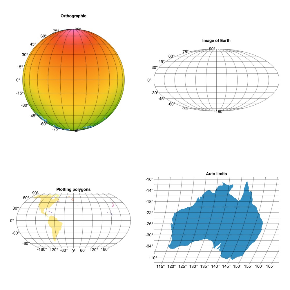
See the documentation for examples and basic usage!
