```@cardmeta
Title = "Raster warping, masking, plotting"
Description = "Semi involved example showing raster warping and masking, and plotting matrix lookup gridded data on a globe."
Cover = fig
```

using CairoMakie, GeoMakie
using Rasters, ArchGDAL,NaturalEarth, FileIO
Background setup

Set up the background. First, load the image,
blue_marble_image = FileIO.load(FileIO.query(download("https://eoimages.gsfc.nasa.gov/images/imagerecords/76000/76487/world.200406.3x5400x2700.jpg"))) |> rotr90 .|> RGBA{Makie.Colors.N0f8}5400×2700 Array{RGBA{N0f8},2} with eltype RGBA{FixedPointNumbers.N0f8}:
RGBA{N0f8}(0.929,0.929,0.929,1.0) … RGBA{N0f8}(0.043,0.055,0.114,1.0)
RGBA{N0f8}(0.929,0.929,0.929,1.0) RGBA{N0f8}(0.043,0.055,0.114,1.0)
RGBA{N0f8}(0.929,0.929,0.929,1.0) RGBA{N0f8}(0.047,0.059,0.118,1.0)
RGBA{N0f8}(0.929,0.929,0.929,1.0) RGBA{N0f8}(0.043,0.055,0.114,1.0)
RGBA{N0f8}(0.929,0.929,0.929,1.0) RGBA{N0f8}(0.039,0.051,0.11,1.0)
RGBA{N0f8}(0.929,0.929,0.929,1.0) … RGBA{N0f8}(0.039,0.051,0.11,1.0)
RGBA{N0f8}(0.929,0.929,0.929,1.0) RGBA{N0f8}(0.039,0.051,0.11,1.0)
RGBA{N0f8}(0.929,0.929,0.929,1.0) RGBA{N0f8}(0.039,0.051,0.11,1.0)
RGBA{N0f8}(0.918,0.918,0.918,1.0) RGBA{N0f8}(0.039,0.051,0.11,1.0)
RGBA{N0f8}(0.918,0.918,0.918,1.0) RGBA{N0f8}(0.039,0.051,0.11,1.0)
⋮ ⋱
RGBA{N0f8}(0.925,0.925,0.925,1.0) RGBA{N0f8}(0.49,0.502,0.522,1.0)
RGBA{N0f8}(0.929,0.929,0.929,1.0) RGBA{N0f8}(0.502,0.502,0.533,1.0)
RGBA{N0f8}(0.929,0.929,0.929,1.0) RGBA{N0f8}(0.502,0.502,0.533,1.0)
RGBA{N0f8}(0.929,0.929,0.929,1.0) RGBA{N0f8}(0.502,0.502,0.533,1.0)
RGBA{N0f8}(0.929,0.929,0.929,1.0) … RGBA{N0f8}(0.502,0.502,0.533,1.0)
RGBA{N0f8}(0.929,0.929,0.929,1.0) RGBA{N0f8}(0.498,0.502,0.522,1.0)
RGBA{N0f8}(0.929,0.929,0.929,1.0) RGBA{N0f8}(0.498,0.502,0.522,1.0)
RGBA{N0f8}(0.929,0.929,0.929,1.0) RGBA{N0f8}(0.502,0.506,0.525,1.0)
RGBA{N0f8}(0.929,0.929,0.929,1.0) RGBA{N0f8}(0.506,0.51,0.529,1.0)Your other choice is:
blue_marble_image = GeoMakie.earth() |> rotr90 .|> RGBA{Makie.Colors.N0f8}720×360 Array{RGBA{N0f8},2} with eltype RGBA{FixedPointNumbers.N0f8}:
RGBA{N0f8}(0.941,0.949,0.965,1.0) … RGBA{N0f8}(0.463,0.659,0.8,1.0)
RGBA{N0f8}(0.941,0.949,0.965,1.0) RGBA{N0f8}(0.463,0.659,0.8,1.0)
RGBA{N0f8}(0.941,0.949,0.965,1.0) RGBA{N0f8}(0.463,0.663,0.8,1.0)
RGBA{N0f8}(0.941,0.949,0.965,1.0) RGBA{N0f8}(0.463,0.663,0.8,1.0)
RGBA{N0f8}(0.941,0.949,0.965,1.0) RGBA{N0f8}(0.463,0.663,0.8,1.0)
RGBA{N0f8}(0.941,0.949,0.965,1.0) … RGBA{N0f8}(0.463,0.663,0.8,1.0)
RGBA{N0f8}(0.941,0.949,0.965,1.0) RGBA{N0f8}(0.463,0.663,0.8,1.0)
RGBA{N0f8}(0.941,0.953,0.965,1.0) RGBA{N0f8}(0.467,0.663,0.8,1.0)
RGBA{N0f8}(0.941,0.953,0.965,1.0) RGBA{N0f8}(0.467,0.663,0.8,1.0)
RGBA{N0f8}(0.945,0.953,0.965,1.0) RGBA{N0f8}(0.467,0.663,0.8,1.0)
⋮ ⋱
RGBA{N0f8}(0.941,0.949,0.961,1.0) RGBA{N0f8}(0.463,0.659,0.796,1.0)
RGBA{N0f8}(0.941,0.949,0.961,1.0) RGBA{N0f8}(0.463,0.659,0.8,1.0)
RGBA{N0f8}(0.941,0.949,0.961,1.0) RGBA{N0f8}(0.463,0.659,0.8,1.0)
RGBA{N0f8}(0.941,0.949,0.961,1.0) RGBA{N0f8}(0.463,0.659,0.8,1.0)
RGBA{N0f8}(0.941,0.949,0.961,1.0) … RGBA{N0f8}(0.463,0.659,0.8,1.0)
RGBA{N0f8}(0.941,0.949,0.961,1.0) RGBA{N0f8}(0.463,0.659,0.8,1.0)
RGBA{N0f8}(0.941,0.949,0.965,1.0) RGBA{N0f8}(0.463,0.659,0.8,1.0)
RGBA{N0f8}(0.941,0.949,0.965,1.0) RGBA{N0f8}(0.463,0.659,0.796,1.0)
RGBA{N0f8}(0.941,0.949,0.965,1.0) RGBA{N0f8}(0.463,0.659,0.8,1.0)For the purposes of this example, we'll use the Natural Earth background image, since it's significantly smaller and the poor CI machine can't handle huge images.
We wrap the image as a Raster for easy masking.
blue_marble_raster = Raster(
    blue_marble_image, # the contents
    ( # the dimensions go in this tuple.  `X` and `Y` are defined by the Rasters ecosystem.
        X(LinRange(-180, 180, size(blue_marble_image, 1))),
        Y(LinRange(-90, 90, size(blue_marble_image, 2)))
    )
)
╭────────────────────────────────────────────────╮
│ 720×360 Raster{RGBA{FixedPointNumbers.N0f8},2} │
├────────────────────────────────────────────────┴─────────────────────── dims ┐
↓ X Sampled{Float64} LinRange{Float64}(-180.0, 180.0, 720) ForwardOrdered Regular Points,
→ Y Sampled{Float64} LinRange{Float64}(-90.0, 90.0, 360) ForwardOrdered Regular Points
├────────────────────────────────────────────────────────────────────── raster ┤
extent: Extent(X = (-180.0, 180.0), Y = (-90.0, 90.0))
└──────────────────────────────────────────────────────────────────────────────┘
↓ → … 90.0
-180.0 RGBA{N0f8}(0.463,0.659,0.8,1.0)
-179.499 RGBA{N0f8}(0.463,0.659,0.8,1.0)
-178.999 RGBA{N0f8}(0.463,0.663,0.8,1.0)
-178.498 RGBA{N0f8}(0.463,0.663,0.8,1.0)
⋮ ⋱ ⋮
177.997 RGBA{N0f8}(0.463,0.659,0.8,1.0)
178.498 RGBA{N0f8}(0.463,0.659,0.8,1.0)
178.999 RGBA{N0f8}(0.463,0.659,0.8,1.0)
179.499 RGBA{N0f8}(0.463,0.659,0.796,1.0)
180.0 … RGBA{N0f8}(0.463,0.659,0.8,1.0)Construct a mask of land using Natural Earth land polygons
land_mask = Rasters.boolmask(NaturalEarth.naturalearth("land", 10); to = blue_marble_raster)╭────────────────────────╮
│ 720×360 Raster{Bool,2} │
├────────────────────────┴─────────────────────────────────────────────── dims ┐
↓ X Sampled{Float64} LinRange{Float64}(-180.0, 180.0, 720) ForwardOrdered Regular Points,
→ Y Sampled{Float64} LinRange{Float64}(-90.0, 90.0, 360) ForwardOrdered Regular Points
├────────────────────────────────────────────────────────────────────── raster ┤
extent: Extent(X = (-180.0, 180.0), Y = (-90.0, 90.0))
missingval: false
└──────────────────────────────────────────────────────────────────────────────┘
↓ → -90.0 -89.4986 -88.9972 … 88.4958 88.9972 89.4986 90.0
-180.0 0 1 1 0 0 0 0
-179.499 0 1 1 0 0 0 0
-178.999 0 1 1 0 0 0 0
-178.498 0 1 1 0 0 0 0
⋮ ⋱ ⋮
177.997 0 1 1 0 0 0 0
178.498 0 1 1 0 0 0 0
178.999 0 1 1 0 0 0 0
179.499 0 1 1 0 0 0 0
180.0 0 0 0 … 0 0 0 0land_raster = deepcopy(blue_marble_raster)
land_raster[(!).(land_mask)] .= RGBA{Makie.Colors.N0f8}(0.0, 0.0, 0.0, 0.0)
land_raster
sea_raster = deepcopy(blue_marble_raster)
sea_raster[land_mask] .= RGBA{Makie.Colors.N0f8}(0.0, 0.0, 0.0, 0.0)
sea_raster╭────────────────────────────────────────────────╮
│ 720×360 Raster{RGBA{FixedPointNumbers.N0f8},2} │
├────────────────────────────────────────────────┴─────────────────────── dims ┐
↓ X Sampled{Float64} LinRange{Float64}(-180.0, 180.0, 720) ForwardOrdered Regular Points,
→ Y Sampled{Float64} LinRange{Float64}(-90.0, 90.0, 360) ForwardOrdered Regular Points
├────────────────────────────────────────────────────────────────────── raster ┤
extent: Extent(X = (-180.0, 180.0), Y = (-90.0, 90.0))
└──────────────────────────────────────────────────────────────────────────────┘
↓ → … 90.0
-180.0 RGBA{N0f8}(0.463,0.659,0.8,1.0)
-179.499 RGBA{N0f8}(0.463,0.659,0.8,1.0)
-178.999 RGBA{N0f8}(0.463,0.663,0.8,1.0)
-178.498 RGBA{N0f8}(0.463,0.663,0.8,1.0)
⋮ ⋱ ⋮
177.997 RGBA{N0f8}(0.463,0.659,0.8,1.0)
178.498 RGBA{N0f8}(0.463,0.659,0.8,1.0)
178.999 RGBA{N0f8}(0.463,0.659,0.8,1.0)
179.499 RGBA{N0f8}(0.463,0.659,0.796,1.0)
180.0 … RGBA{N0f8}(0.463,0.659,0.8,1.0)Constructing fake data
Now, we construct fake data.
field = [exp(cosd(x)) + 3(y/90) for x in -180:180, y in -90:90]

ras = Raster(field, (X(LinRange(-30, 30, size(field, 1))), Y(LinRange(-5, 5, size(field, 2)))); missingval = NaN)
╭───────────────────────────╮
│ 361×181 Raster{Float64,2} │
├───────────────────────────┴──────────────────────────────────────────── dims ┐
↓ X Sampled{Float64} LinRange{Float64}(-30.0, 30.0, 361) ForwardOrdered Regular Points,
→ Y Sampled{Float64} LinRange{Float64}(-5.0, 5.0, 181) ForwardOrdered Regular Points
├────────────────────────────────────────────────────────────────────── raster ┤
extent: Extent(X = (-30.0, 30.0), Y = (-5.0, 5.0))
missingval: NaN
└──────────────────────────────────────────────────────────────────────────────┘
↓ → -5.0 -4.94444 … 4.83333 4.88889 4.94444 5.0
-30.0 -2.63212 -2.59879 3.26788 3.30121 3.33455 3.36788
-29.8333 -2.63206 -2.59873 3.26794 3.30127 3.3346 3.36794
-29.6667 -2.6319 -2.59856 3.2681 3.30144 3.33477 3.3681
-29.5 -2.63162 -2.59828 3.26838 3.30172 3.33505 3.36838
⋮ ⋱ ⋮
29.3333 -2.63122 -2.59789 3.26878 3.30211 3.33544 3.36878
29.5 -2.63162 -2.59828 3.26838 3.30172 3.33505 3.36838
29.6667 -2.6319 -2.59856 3.2681 3.30144 3.33477 3.3681
29.8333 -2.63206 -2.59873 … 3.26794 3.30127 3.3346 3.36794
30.0 -2.63212 -2.59879 3.26788 3.30121 3.33455 3.36788We rotate the raster and then translate it to approximate the position in the image.
rotmat = Makie.rotmatrix2d(-π/5)

transformed = Rasters.warp(
    ras,
    Dict(
        "r" => "bilinear",
        "ct" => #= see https://gdal.org/en/latest/programs/gdalwarp.html =# """
        +proj=pipeline
        +step +proj=affine +xoff=$(30) +yoff=$(-36) +s11=$(rotmat[1,1]) +s12=$(rotmat[1,2]) +s21=$(rotmat[2,1]) +s22=$(rotmat[2,2])
        """,
        "s_srs" => "+proj=longlat +datum=WGS84 +type=crs",
        "t_srs" => "+proj=longlat +datum=WGS84 +type=crs",
    )
)
╭───────────────────────────╮
│ 361×288 Raster{Float64,2} │
├───────────────────────────┴──────────────────────────────────────────── dims ┐
↓ X Projected{Float64} LinRange{Float64}(2.7823459563862345, 57.16214601458978, 361) ForwardOrdered Regular Points,
→ Y Projected{Float64} LinRange{Float64}(-57.678215207187165, -14.32543016078601, 288) ForwardOrdered Regular Points
├──────────────────────────────────────────────────────────────────── metadata ┤
Metadata{Rasters.GDALsource} of Dict{String, Any} with 4 entries:
"units" => ""
"offset" => 0.0
"filepath" => "/vsimem/tmp"
"scale" => 1.0
├────────────────────────────────────────────────────────────────────── raster ┤
extent: Extent(X = (2.7823459563862345, 57.16214601458978), Y = (-57.678215207187165, -14.32543016078601))
missingval: NaN
crs: GEOGCS["unknown",DATUM["WGS_1984",SPHEROID["WGS 84",6378137,298.257223563,AUTHORITY["EPSG","7030"]],AUTHORITY["EPSG","6326"]],PRIMEM["Greenwich",0,AUTHORITY["EPSG","8901"]],UNIT["degree",0.0174532925199433,AUTHORITY["EPSG","9122"]],AXIS["Longitude",EAST],AXIS["Latitude",NORTH]]
└──────────────────────────────────────────────────────────────────────────────┘
↓ → -57.6782 -57.5272 -57.3761 … -14.6275 -14.4765 -14.3254
2.78235 NaN NaN NaN NaN NaN NaN
⋮ ⋱
57.1621 NaN NaN NaN NaN NaN NaNPlotting the data
fig = Figure(size = (1000, 1000))
ax = GeoAxis(fig[1, 1]; dest = "+proj=ortho +lon_0=0 +lat_0=0")

sea_plot = meshimage!(ax, sea_raster; source = "+proj=longlat +datum=WGS84 +type=crs", npoints = 300)

land_plot = meshimage!(ax, land_raster; source = "+proj=longlat +datum=WGS84 +type=crs", npoints = 300)

data_plot = surface!(ax, transformed; shading = NoShading)
Surface{Tuple{Vector{Float64}, Vector{Float64}, Matrix{Float32}}}Get the land plot above all other plots in the geoaxis.
translate!(land_plot, 0, 0, 1)3-element Vec{3, Float64} with indices SOneTo(3):
0.0
0.0
1.0Display the figure...
fig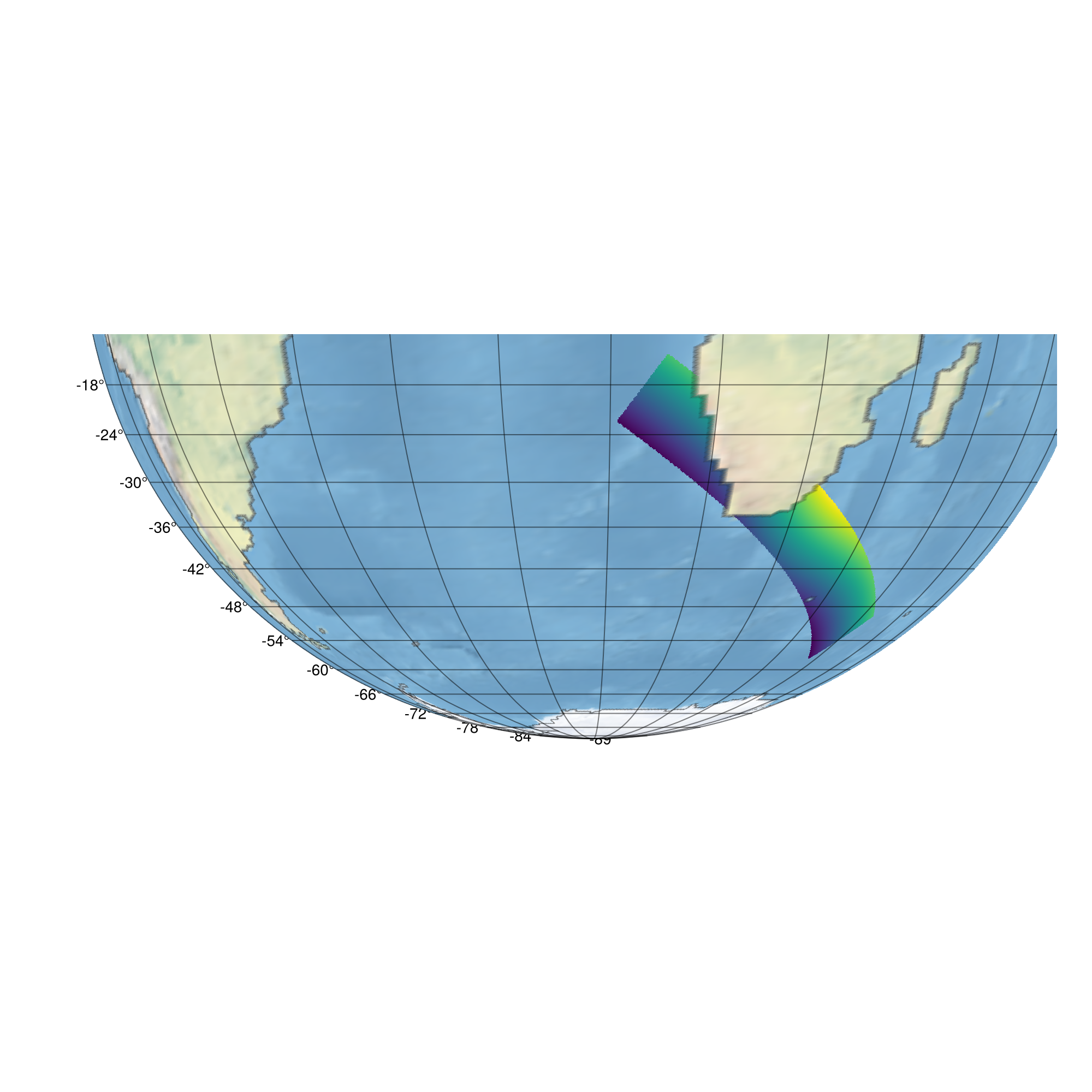
For extra credit, we'll find the center of the raster and transform the orthographic projection to be centered on it:
xy_matrix = Rasters.DimensionalData.DimPoints(transformed) |> collect
center_x = mean(first.(xy_matrix))
center_y = mean(last.(xy_matrix))
We'll use the ortho projection, which is centered on the point we just found.
ax.dest = "+proj=ortho +lon_0=$(center_x) +lat_0=$(center_y)"

fig
Plotting on the 3D globe
Super bonus points: plot the data on the globe
using Geodesyfig = Figure(size = (1000, 1000));
fig = Figure()

ax = LScene(fig[1, 1])

sea_plot = meshimage!(ax, sea_raster; npoints = 300)

land_plot = meshimage!(ax, land_raster; npoints = 300)

data_plot = surface!(ax, transformed; shading = NoShading)

land_plot.z_level[] = 1000

sea_plot.transformation.transform_func[] = Geodesy.ECEFfromLLA(Geodesy.WGS84())
land_plot.transformation.transform_func[] = Geodesy.ECEFfromLLA(Geodesy.WGS84())
data_plot.transformation.transform_func[] = Geodesy.ECEFfromLLA(Geodesy.WGS84())

fig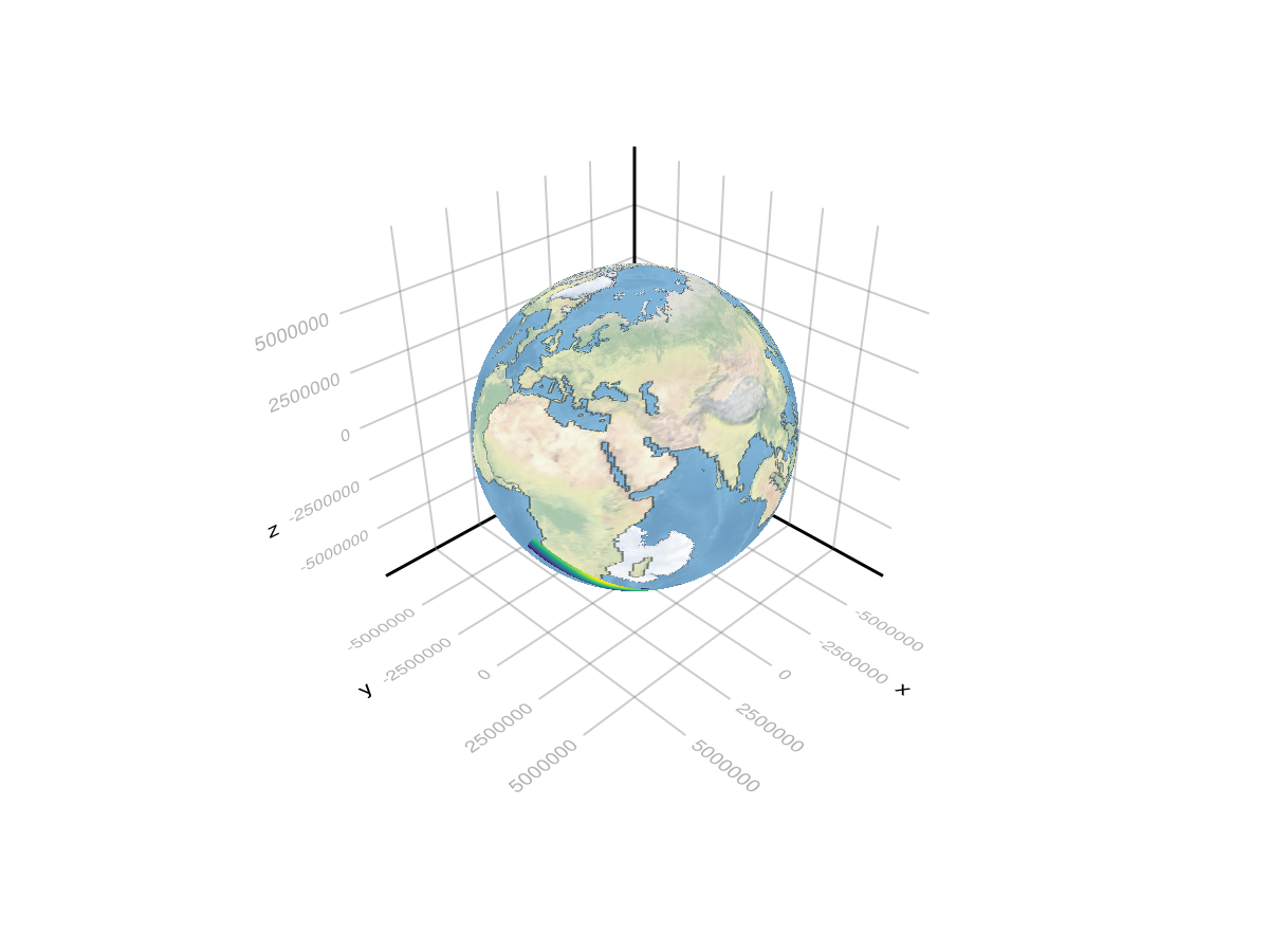
This page was generated using Literate.jl.