Histogram

You can use any Makie compatible recipe in GeoMakie, and this includes histograms! Until we get the datashader recipe working, you can also consider this a replacement for that if you use it with the correct nbins.

We use the excellent FHist.jl to create the histogram.

using CairoMakie, GeoMakie
using FHist
import CairoMakie: Point2d

First, we generate random points in a normal distribution:

random_data = randn(Point2d, 100_000)

100000-element Vector{GeometryBasics.Point{2, Float64}}:
 [-1.7337637961618357, -0.47452167542324303]
 [1.4532771738043138, -0.6324680476859472]
 [-0.4817002804091031, -0.3724485335613098]
 [0.1682928011687825, 0.24889814372319916]
 [0.0658431760448007, -1.8865111591873744]
 [-1.5330248091153387, 0.3317588760378498]
 [0.5667003736572725, 0.7923524952104092]
 [0.6128647716581239, 0.1576743017288308]
 [0.23269286685896887, -0.9131038790059479]
 [-0.11476351849141027, -0.11880269424380976]
 ⋮
 [0.49733941529526055, 1.0332427327271505]
 [-0.6071502942676916, 1.1746456607810727]
 [-2.3108457162095717, -0.961740526847832]
 [-0.02915309682318518, 0.6779039369431118]
 [0.6545560901430979, 0.9363853243128094]
 [-0.09806119173232478, -0.42603982506272847]
 [-1.0070954284508622, 0.16493162880749082]
 [1.5813897473835272, -0.3762185913148442]
 [-0.8234520311747406, -1.4979478699757274]

then, we rescale them to be within the lat/long bounds of the Earth:

xmin, xmax = extrema(first, random_data)
ymin, ymax = extrema(last, random_data)
latlong_data = random_data .* (Point2d(1/(xmax - xmin), 1/(ymax - ymin)) * Point2d(360, 180),)

100000-element Vector{GeometryBasics.Point{2, Float64}}:
 [-66.76446102923026, -9.245182920872068]
 [55.963371394606696, -12.322477760890518]
 [-18.54950465013683, -7.256475309191337]
 [6.4806856562624695, 4.849322984738348]
 [2.535515028526704, -36.75520350761069]
 [-59.03432483225664, 6.463712098835363]
 [21.822721812538934, 15.43753243620708]
 [23.600438683827218, 3.071994045590469]
 [8.960628821283416, -17.790151271042085]
 [-4.41935889701892, -2.3146521996003577]
 ⋮
 [19.151742633159213, 20.13083608289126]
 [-23.38038333148883, 22.885812310772522]
 [-88.98695953046442, -18.737746985305698]
 [-1.1226389667622523, 13.207712575465221]
 [25.205904442432466, 18.243747453623694]
 [-3.776179101436003, -8.300603151095446]
 [-38.78162852077878, 3.2133897285146795]
 [60.89678097728401, -7.329927957107977]
 [-31.709816046749825, -29.18476179513621]

finally, we can create the histogram.

h = Hist2D((first.(latlong_data), last.(latlong_data)); nbins = (360, 180))

<rect x="38" y="10" width="200" height="160.0" fill="none" stroke="#000" stroke-width="1" /> <text x="37.5" y="185.0" fill="black" dominant-baseline="middle" text-anchor="middle" font-size="85%" font-family="sans-serif" >-187.0</text> <text x="237.5" y="185.0" fill="black" dominant-baseline="middle" text-anchor="middle" font-size="85%" font-family="sans-serif" >174.0</text> <text x="18.75" y="170.0" fill="black" dominant-baseline="middle" text-anchor="middle" font-size="85%" font-family="sans-serif" >-89.0</text> <text x="18.75" y="10.0" fill="black" dominant-baseline="middle" text-anchor="middle" font-size="85%" font-family="sans-serif" >92.0</text> 

• edges: ([-187.0, -186.0, -185.0, -184.0, -183.0, -182.0, -181.0, -180.0, -179.0, -178.0 … 165.0, 166.0, 167.0, 168.0, 169.0, 170.0, 171.0, 172.0, 173.0, 174.0], [-89.0, -88.0, -87.0, -86.0, -85.0, -84.0, -83.0, -82.0, -81.0, -80.0 … 83.0, 84.0, 85.0, 86.0, 87.0, 88.0, 89.0, 90.0, 91.0, 92.0])
• bin counts: [0.0 0.0 … 0.0 0.0; 0.0 0.0 … 0.0 0.0; … ; 0.0 0.0 … 0.0 0.0; 0.0 0.0 … 0.0 0.0]
• maximum count: 41.0
• total count: 100000.0

This is what the histogram looks like without any projection,

plot(h)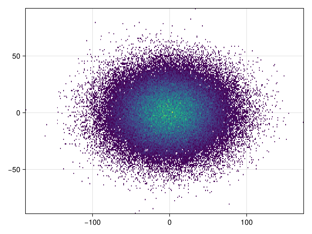

It's simple to plot to GeoAxis:

plot(h; axis = (; type = GeoAxis))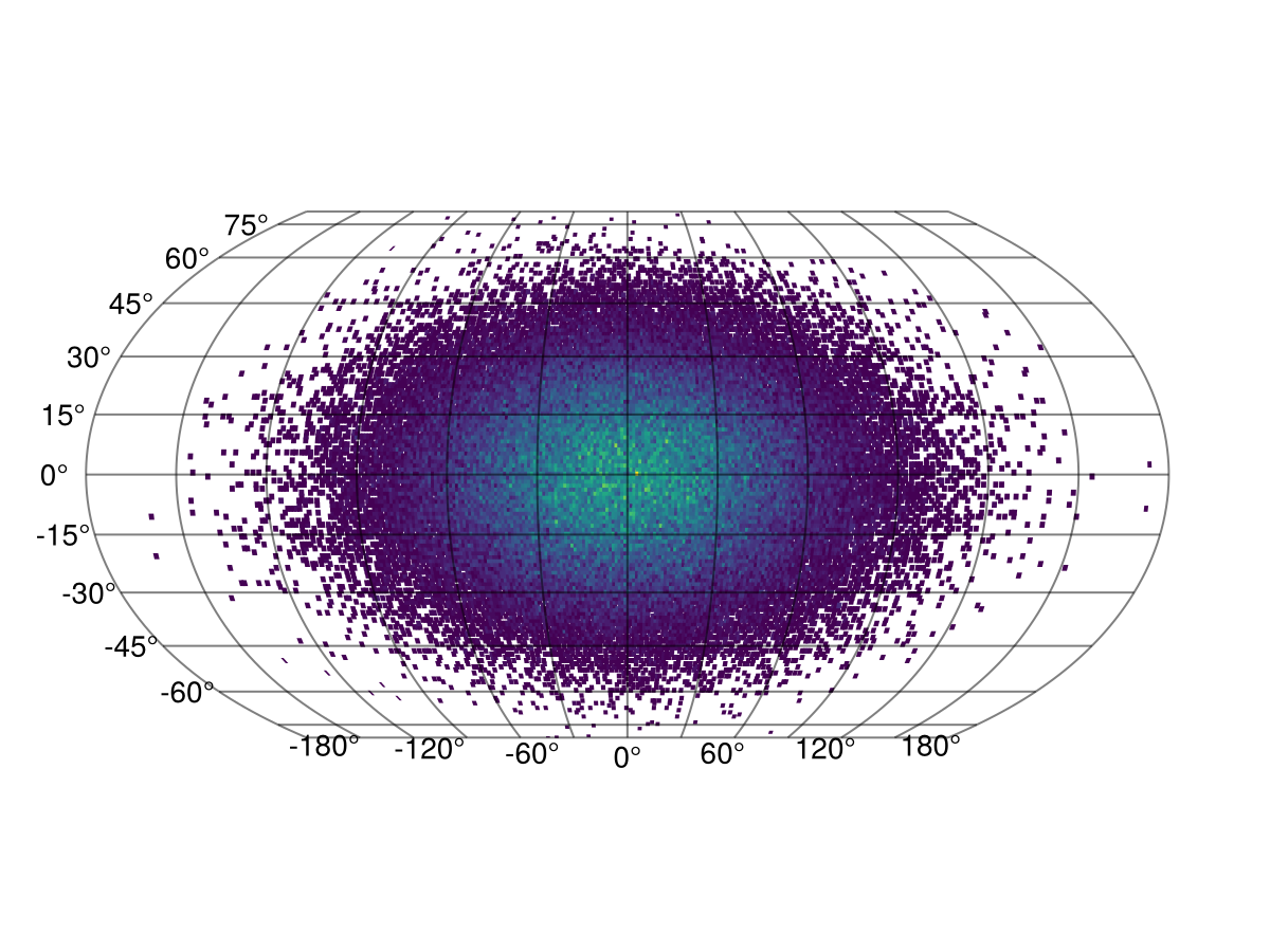

The projection can also be arbitrary!

plot(h; axis = (; type = GeoAxis, dest = "+proj=tissot +lat_1=60 +lat_2=65"))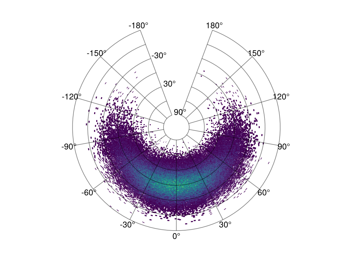

---

This page was generated using Literate.jl.