Raster data (with Rasters.jl)

Rasters.jl is a Julia package designed for working with raster data. It provides tools to read, write, and manipulate raster datasets, which are commonly used in geographic information systems (GIS), remote sensing, and similar fields where grid data is prevalent. It's built on top of DimensionalData.jl, which also underpins e.g. YAXArrays.jl.

In general, any input that works with base Makie will work with GeoMakie in a GeoAxis!

First, we'll load Rasters.jl, RasterDataSources.jl which provides access to common datasets, and ArchGDAL.jl which Rasters.jl depends on to read files.

using Rasters, RasterDataSources, ArchGDAL

We'll also load GeoMakie and CairoMakie to plot the data.

using GeoMakie, CairoMakie

First, we can load a Raster from the EarthEnv project, which represents habitat or ecosystem heterogeneity.

ras = Raster(EarthEnv{HabitatHeterogeneity}, :homogeneity) # habitat homogeneity to neighbouring pixel

╭───────────────────────────────────────╮
│ 1728×696 Raster{UInt16,2} homogeneity │
├───────────────────────────────────────┴──────────────────────────────── dims ┐
  ↓ X Projected{Float64} LinRange{Float64}(-180.0, 179.79166666666669, 1728) ForwardOrdered Regular Intervals{Start},
  → Y Projected{Float64} LinRange{Float64}(84.79166666666667, -60.0, 696) ReverseOrdered Regular Intervals{Start}
├──────────────────────────────────────────────────────────────────── metadata ┤
  Metadata{Rasters.GDALsource} of Dict{String, Any} with 4 entries:
  "units"    => ""
  "offset"   => 0.0
  "filepath" => "/home/runner/.julia/artifacts/EarthEnv/HabitatHeterogeneity/25…
  "scale"    => 1.0
├────────────────────────────────────────────────────────────────────── raster ┤
  extent: Extent(X = (-180.0, 180.00000000000003), Y = (-60.0, 85.0))
  missingval: 0xffff
  crs: GEOGCS["WGS 84",DATUM["WGS_1984",SPHEROID["WGS 84",6378137,298.257223563,AUTHORITY["EPSG","7030"]],AUTHORITY["EPSG","6326"]],PRIMEM["Greenwich",0,AUTHORITY["EPSG","8901"]],UNIT["degree",0.0174532925199433,AUTHORITY["EPSG","9122"]],AXIS["Latitude",NORTH],AXIS["Longitude",EAST],AUTHORITY["EPSG","4326"]]
└──────────────────────────────────────────────────────────────────────────────┘
    ↓ →        84.7917      84.5833  …     -59.5833     -59.7917     -60.0
 -180.0    0xffff       0xffff          0xffff       0xffff       0xffff
    ⋮                                ⋱                    ⋮       
  179.792  0xffff       0xffff          0xffff       0xffff       0xffff

Let's take a look at this in regular Makie first:

heatmap(ras; axis = (; aspect = DataAspect()))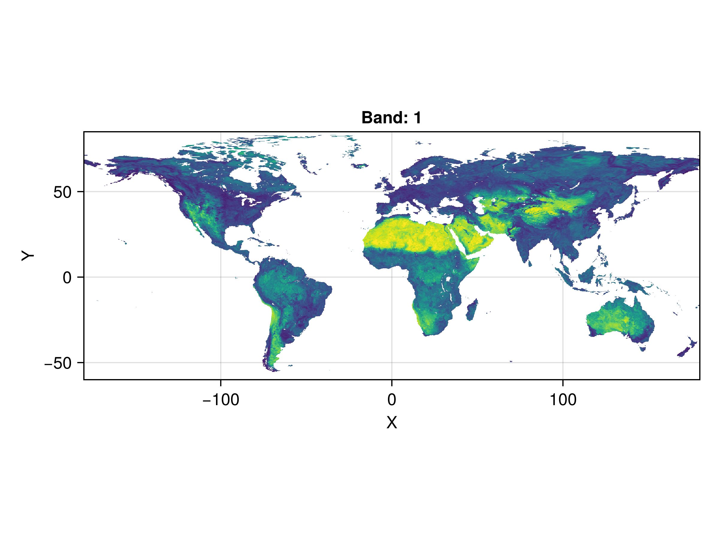

We can plot this in any projection:

fig = Figure(); ga = GeoAxis(fig[1, 1])
hm = heatmap!(ga, ras)
fig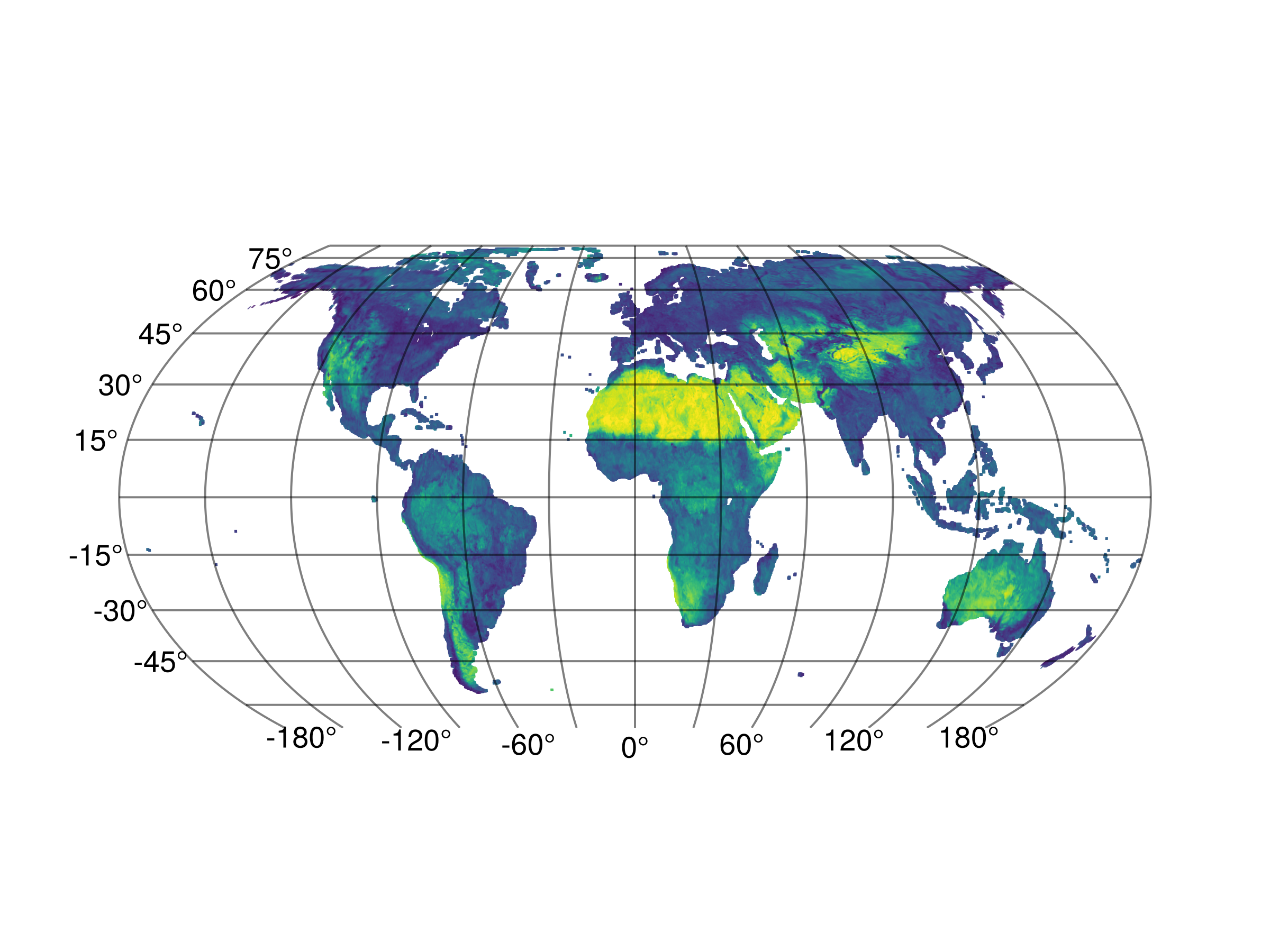

We can also change the projection arbitrarily:

ga.dest[] = "+proj=ortho +lon_0=19 +lat_0=72"
fig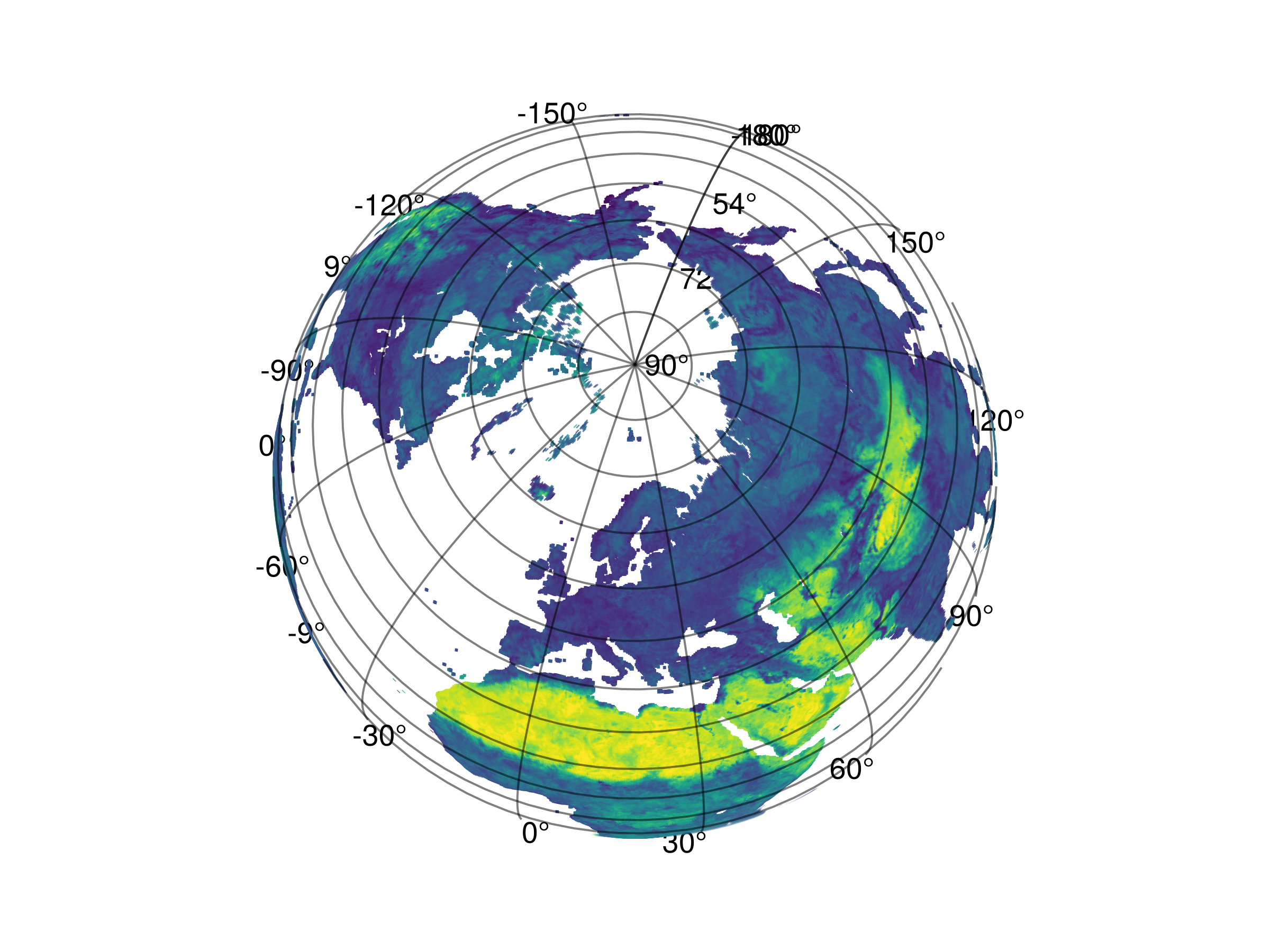

and all other Makie keyword arguments also apply!

hm.colormap = :isoluminant_cgo_70_c39_n256
fig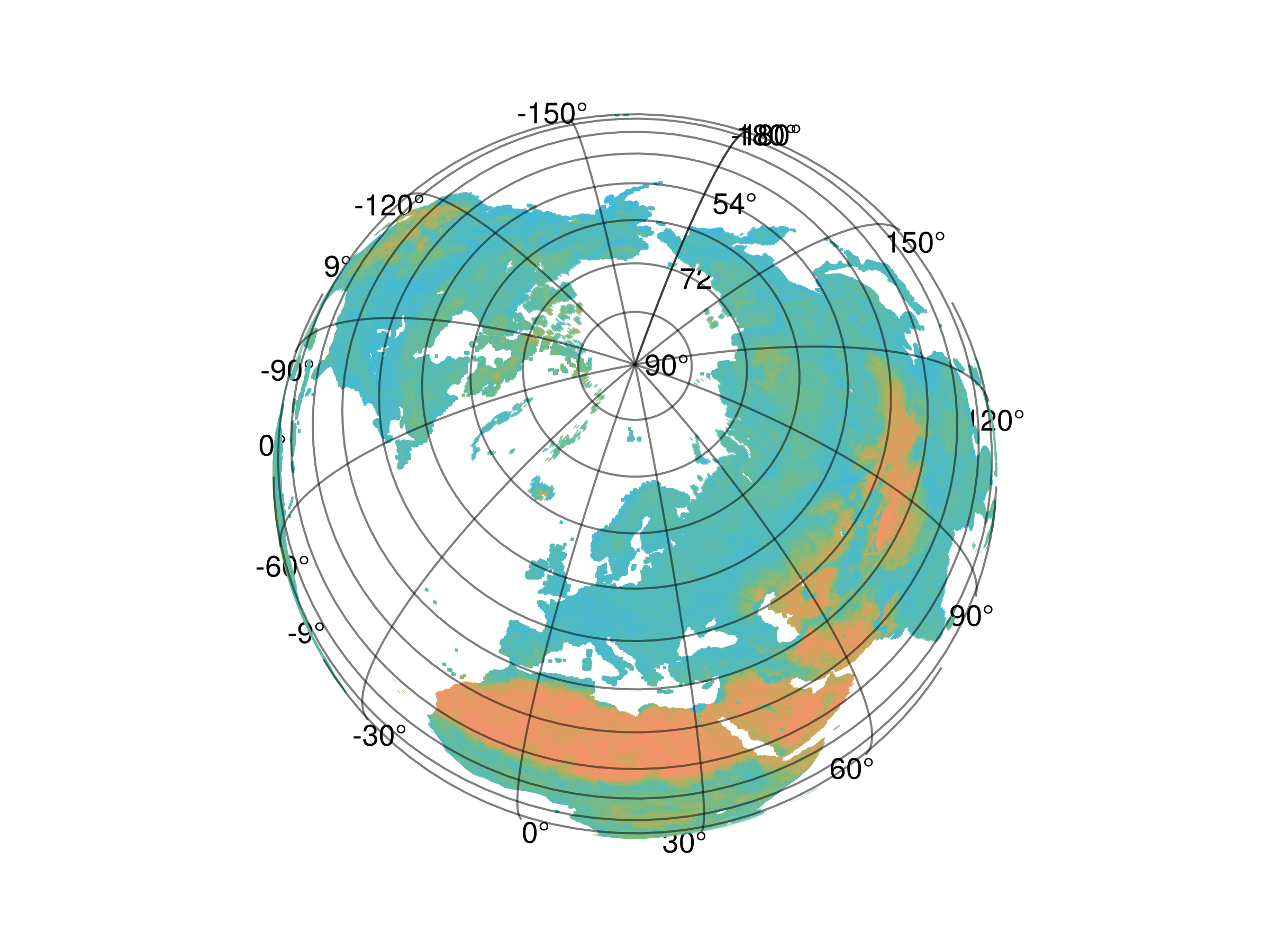

You can also use other recipes like surface:

fig = Figure(); ga = GeoAxis(fig[1, 1])
sp = surface!(ga, ras)
fig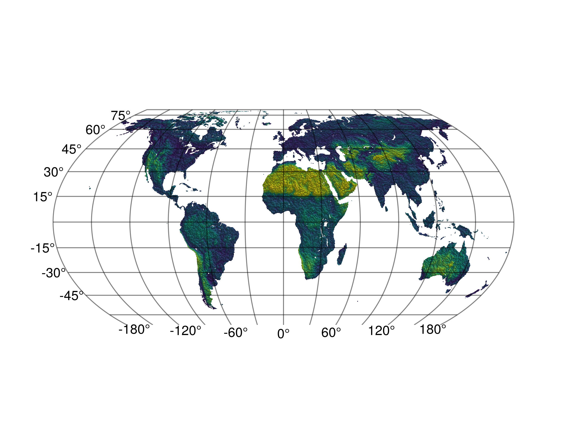

This looks a bit strange - but you can always disable shading:

sp.shading = NoShading
fig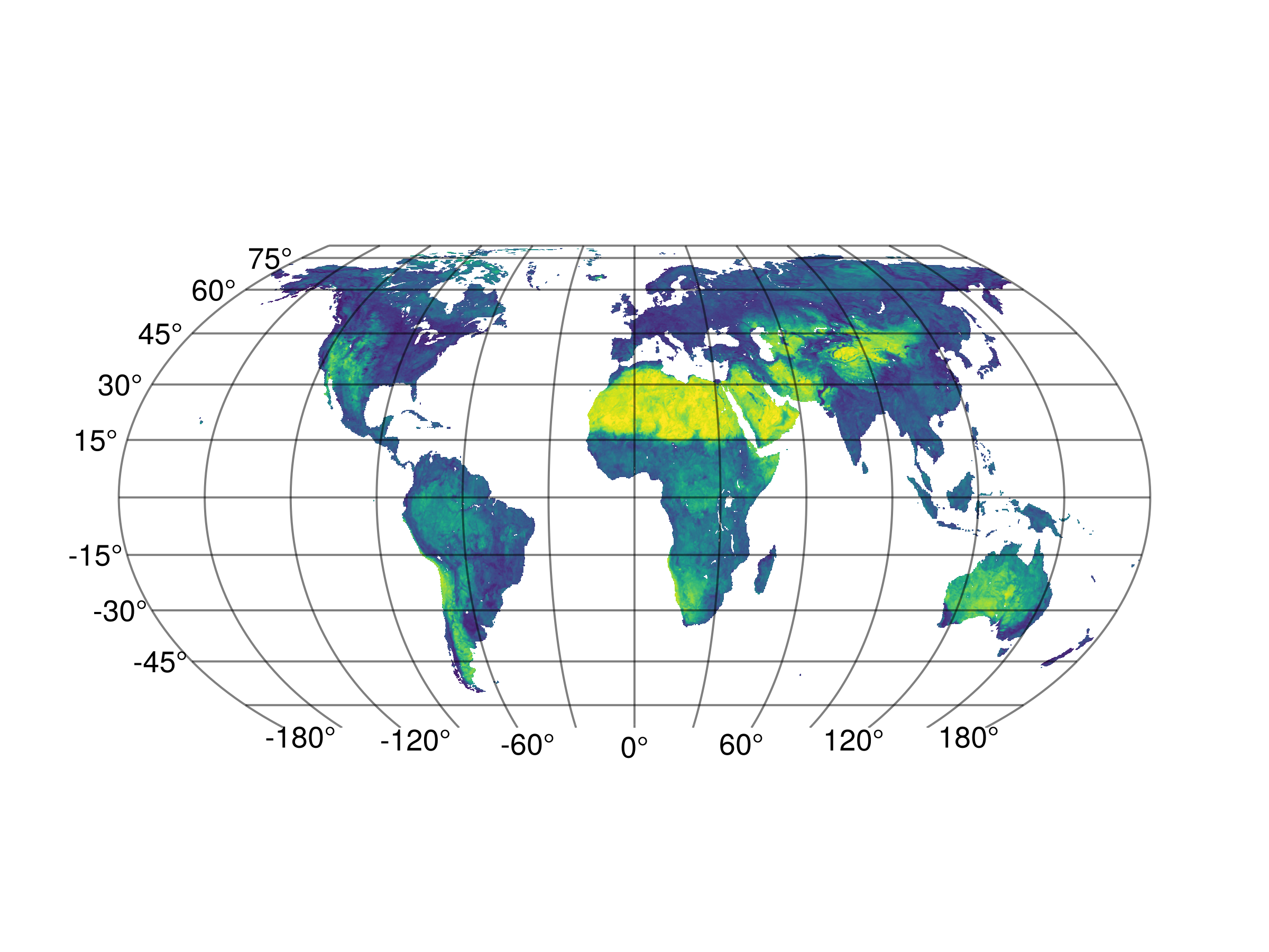

See also the Geostationary image and Multiple CRS examples, where we explore how to plot data in different projections.

---

This page was generated using Literate.jl.